CFD analysis on Cyclone Separator by Ansys fluent

Abstract:

In this project a CFD modelling of a cyclone separator is conducted using discrete phase modelling scheme. The particle injected through the inlet are trapped below and clean air escapes out from the above opening. Turbulent model using k-epsilon is applied with swirl dominating effect. The particle diameter and the velocity of flow is varied in each case to test the efficiency of the cyclone separator.

Aim:-

To perform analysis on cyclone separator and calculate the separation efficiency and pressure drop.

Objective:-

1. To write a few words about any four empirical models used to calculate the cyclone separator efficiency.
2. To perform an analysis on a given cyclone separator model by varying the particle diameter from 1 μm to 5 μm and calculate the separation efficiency in each case. Discuss the results. [Use both the velocity's as 3m/sec.]
3. To perform an analysis on a given cyclone separator model by varying the particle velocity from 1 m/sec to 5 m/sec and calculate the separation efficiency and pressure drop in each case. Discuss the results. [Use particle diameter size as 5 μm for all cases & keep flow velocity same as particle velocity].

Introduction to cyclone seperator and different emperical models to calculate seperator efficiency:-

Cyclones are devices that employ a centrifugal force generated by a spinning gas stream to separate particles from the carrier gas. Their simple design, low capital cost and nearly maintenance-free operation make them ideal for use as precleaners for more expensive final control devices such as bag-30 houses or electrostatic precipitators. Cyclones are particularly well suited for high temperature and pressure conditions be- cause of their rugged design and flexible component materials. Cyclone collection efficiencies can reach 99% for particles bigger than 5 μm.Cyclones are used for the removal of large particles for both air pollution control and process use. Application in extreme conditions includes the removal of coal dust in a power plant and the use as a spray dryer or gasification reactor.
Engineers are generally interested in two parameters in order to carry out an assessment of the design and performance of a cy-clone. These parameters are the collection efficiency of particle and pressure drop through the cyclone. An accurate prediction of cyclone efficiency is very important because an inaccuracy in the efficiency prediction may result in an inefficient design of the cyclone separator. CFD has a great potential to predict the 45 flow field characteristics and particle trajectories inside the cyclone as well as the pressure drop.The complicated swirling turbulent flow in a cyclone places great demands on the numerical techniques and the turbulence models employed in the CFD codes when modelling the cyclone pressure drop.

CYCLONE EFFICIENCY EMPIRICAL MODELS

Iozia and Leith Model

Iozia and Leith [4] logistic model is a modified version of Barth [15] Model, which is developed based on force balance. The model assumes that a particle carried by the vortex endures 165 the influence of two forces: a centrifugal force, Z and a flow resistance, W. The collection efficiency `eta`i of particle diameter dpi can be calculated from

`eta_i = 1 /(1+ (d_c/d_pi )^beta)`

`beta`is an expression for slope parameter derived based on thestatistical analysis of experimental data of a cyclone with D =0.25 m given as

`beta=0.62−0.87 ln (d_(pc)/100 ) +5.21 ln ((ab)/ D^2) +1.05 [ ln ((ab) /D^2)]^2`

and dpc is the 50% cut size given by Barth

`dpc = ((9 μQ )/(pzcv_t^2))^0.5`

where core length, zc, and core diameter, dc, are given as

`zc = (H − S)− (H − S) /((D/B)−1 ) [(d_c/B)−1] for dc > B`

`zc = H − S for dc < B`

`dc = 0.47D ((ab )/D^2 )^(−0.25)((De)/D)^1.4`

Li and Wang Model

The Li and Wang model includes particle bounce or reentrainment and turbulent diffusion at the cyclone wall. A two- dimensional analytical expression of particle distribution in the cyclone is obtained. Li and Wang model was developed based on the following assumption

The radial particle velocity and the radial concentrationprofile are not constant for uncollected particles within the cyclone.

Boundary conditions with the consideration of turbulent diffusion coefficient and particle bounce reentrainment on the cyclone wall are

`c = ctheta , theta = 0`

`Dr (delc/(delr)) = (1 − alpha )wc, at r = D/2`

The tangential velocity is related to the radius of cyclone by: uRn = constant.

The concentration distribution in a cyclone is given as:

`c(r, theta) = (c_0(rw − rn) exp { −lambda(1/( K(1+n)) r^ (1+n))} )/ (int_r exp { 1/( K(1+n)) r^ (1+n)} dr`

where `K = ((1 − n)(rho_p − rho_g)d^2Q)/( 18 μb [ r_w^( 1−n ) − r_n^( 1−n )])`

and `lambda = ((1 − alpha )K W_w) /(D_r r_w^n)`

The resultant expression of the collection efficiency for particle
of any size is given as

`eta_i = 1 − exp{−lambda theta_1}`

where `theta_1 = 2pi(S + L)/a`

Koch and Licht Model
Koch and Licht collection theory recognized the inherently turbulent nature of cyclones and the distribution of gas residence times within the cyclone. Koch and Licht described particle motion in the entry and collection regions with the additional following assumptions:
• The tangential velocity of a particle is equal to the tangential velocity of the gas flow, i.e. there is no slip in the tangential direction between the particle and the gas.
• The tangential velocity is related to the radius of cyclone by: uRn = constant

Aforce balance and an equation on the particles collection yields
the grade efficiency `eta_i = 1 − exp {−2 [ (G tau_i Q (n + 1))/(n+1)] ^(0.5/(n+1) )}`i

`G =( 8K_c )/(K_a^2 K_b^2)`

`n = 1 − { 1 − (12D)^0.14 /2.5} { (T + 460)/ 530 }^0.3`

`tau_i = rho_pd_pi^2 /(18μ)`

Lapple Model
Lapple model was developed based on force balance without considering the flow resistance. Lapple assumed that a particle entering the cyclone is evenly distributed across the inlet opening. The particle that travels from inlet half width to the wall in the cyclone is collected with 50% efficiency. The semi empirical relationship developed by Lapple to calculate a 50% cut diameter, dpc, is

`dpc = [( 9 μb 2)/ (N_ev_i (rho_p − rho_g) )]^(1/2)`

where Ne is the number of revolutions

`Ne = (1 /a) [ h + (H − h) /2 ]`

The efficiency of collection of any size of particle is given by

`eta_i = 1 /((1+ (d_(pc)/d_pi ))^2`

Modelling approach:-

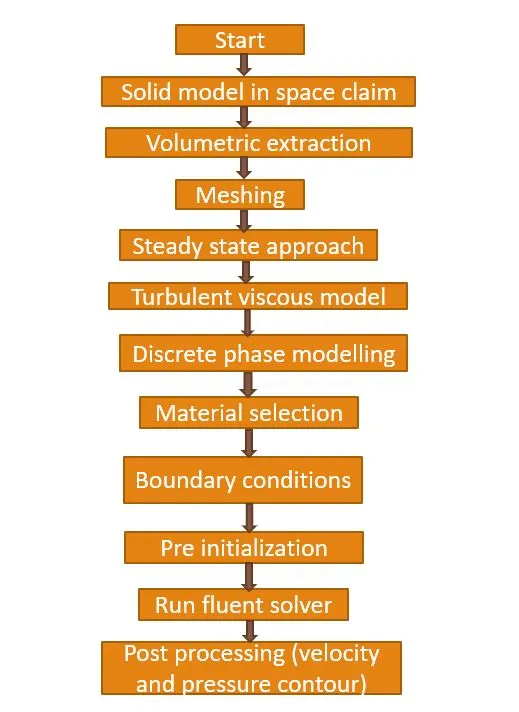
Boundary Conditions:-

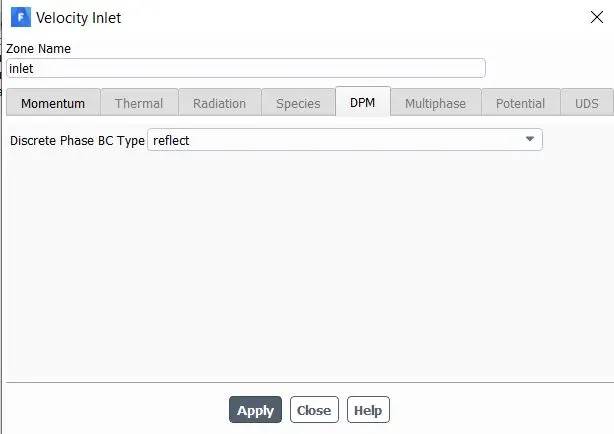
Inlet and wall:- Reflect

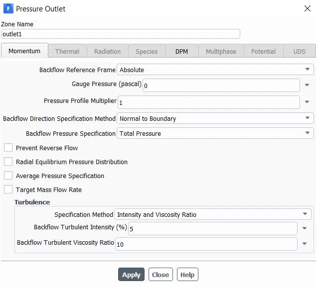
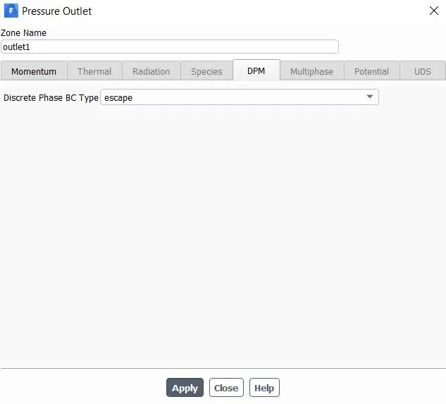
Outlet(Top):- Escape

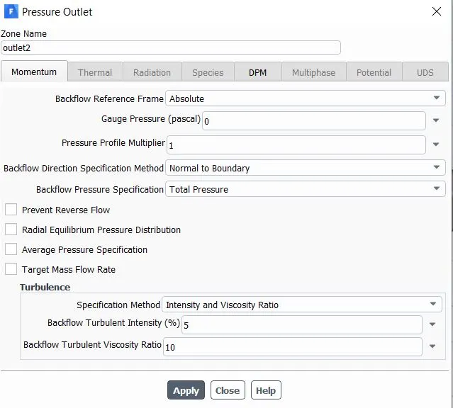
Outlet(Bottom/dustbin) - Trap

Geometry modelling:

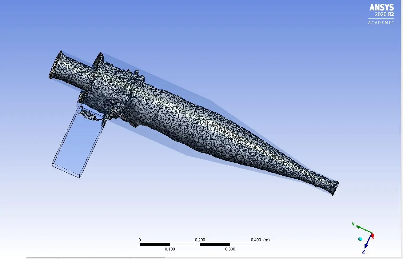
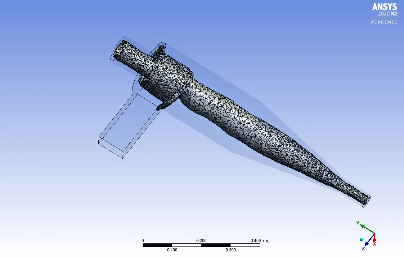
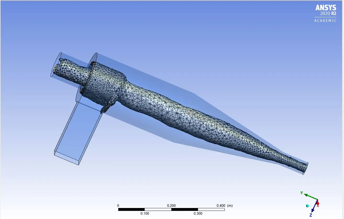
1. Import the cyclone separator model in step format to the space claim design tab.
2. 
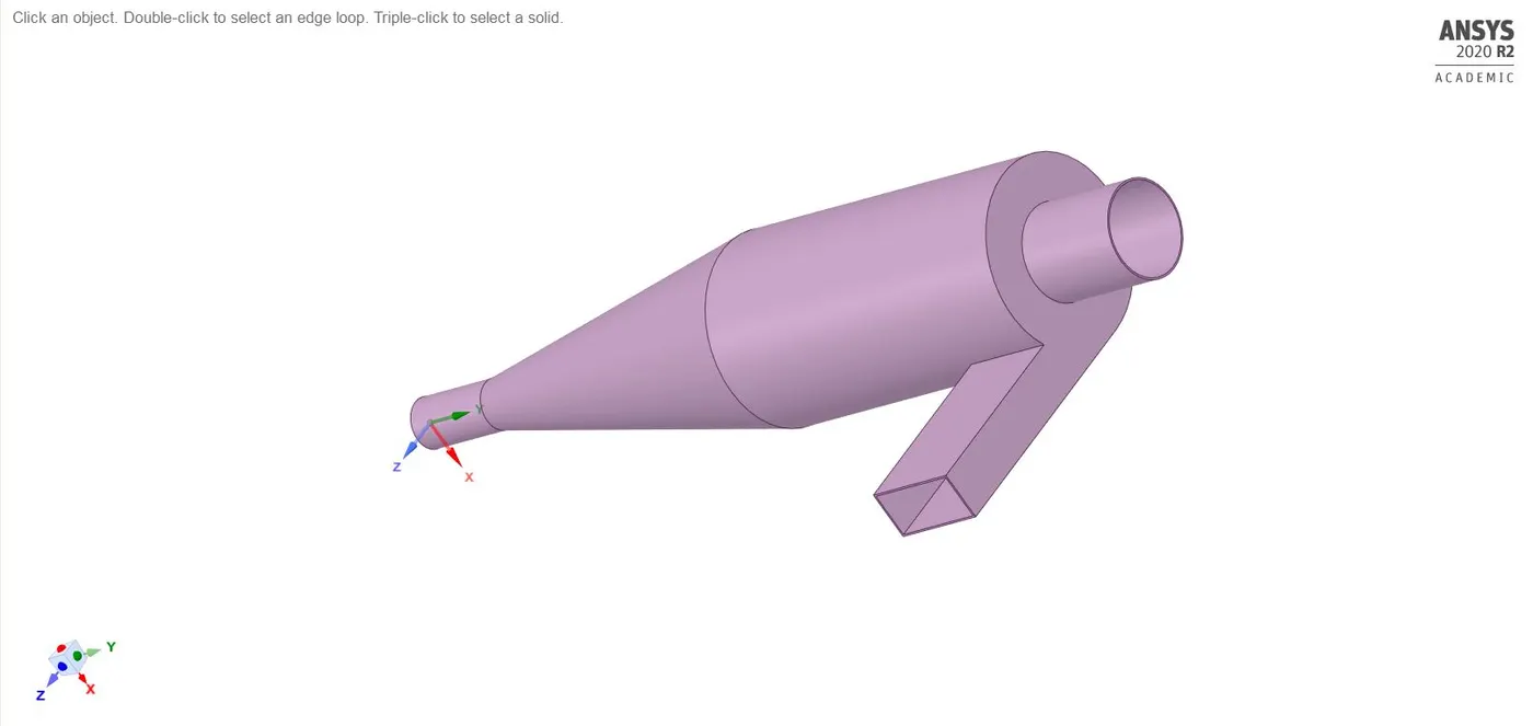
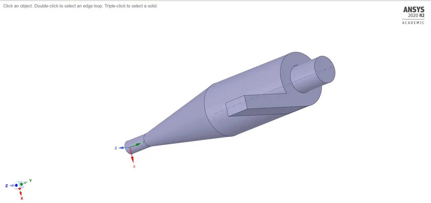
3. Volumetric extraction is done from prepare tool box>> select the edge selection mode and the select the inlet and outlet edges of the model.
4. The final fluid geometrical model is prepared.

Meshing:

1. Open the mesh console.
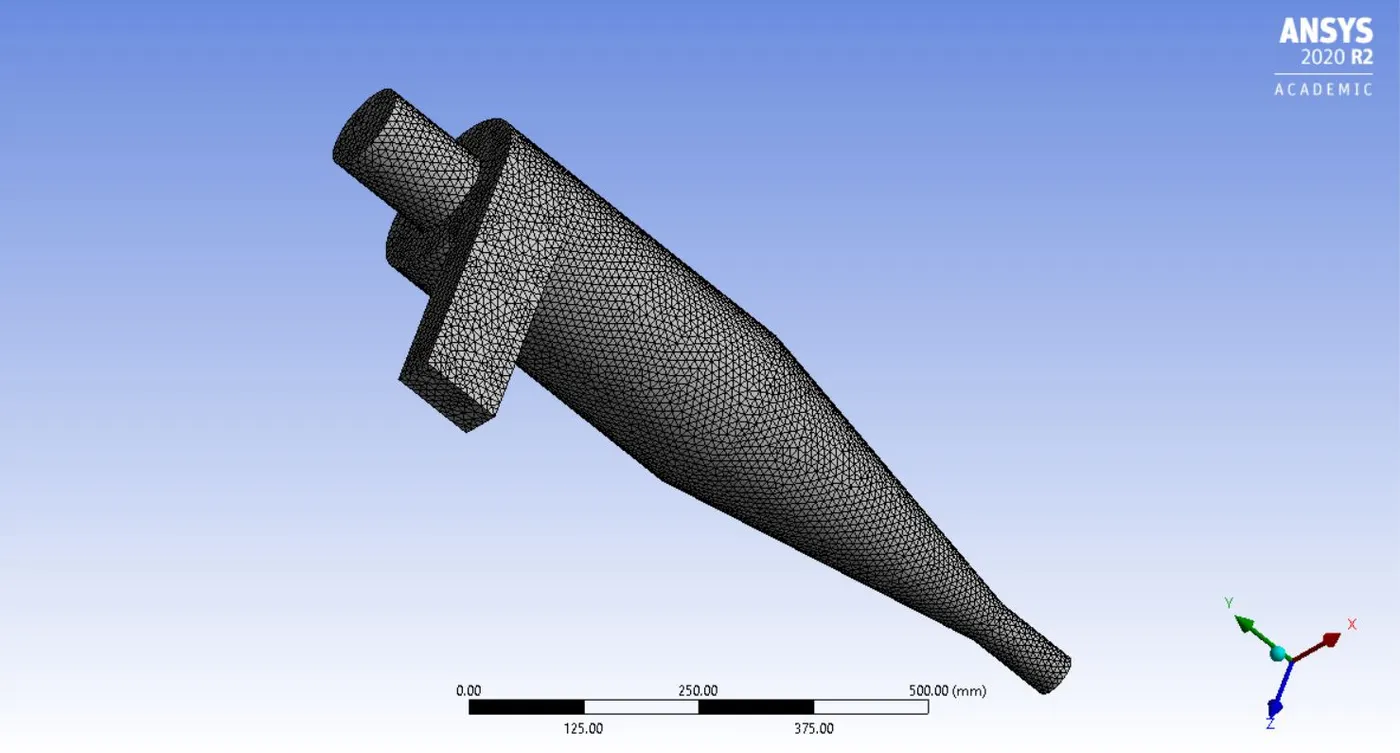
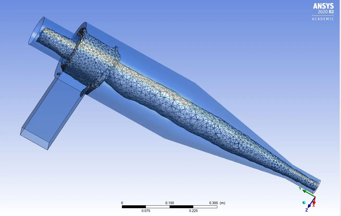
2. Go to mesh settings>> click on the size tab>> give a size of 10mm and click generate option.
3. Provide named selection to inlet and outlet zones.
4. 
5. 
6. 
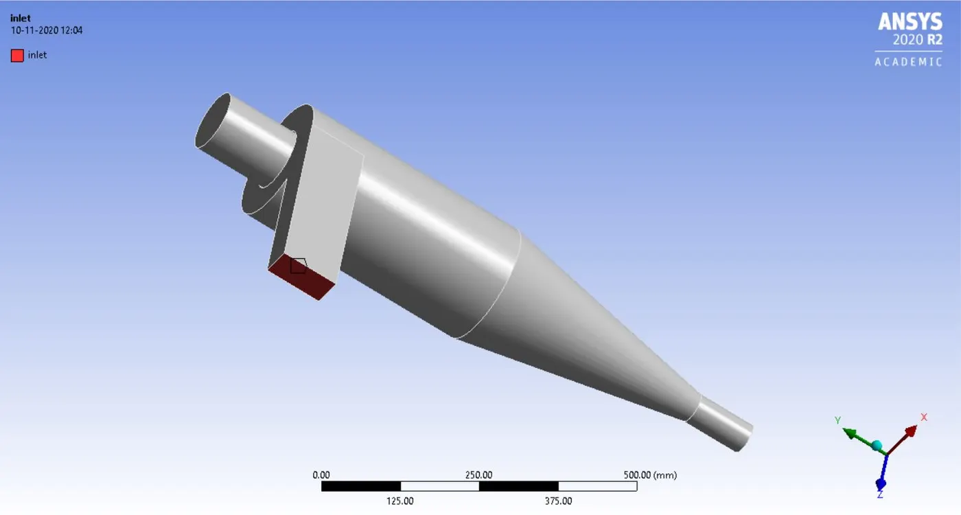
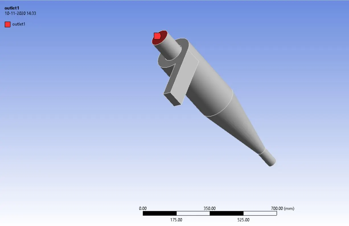
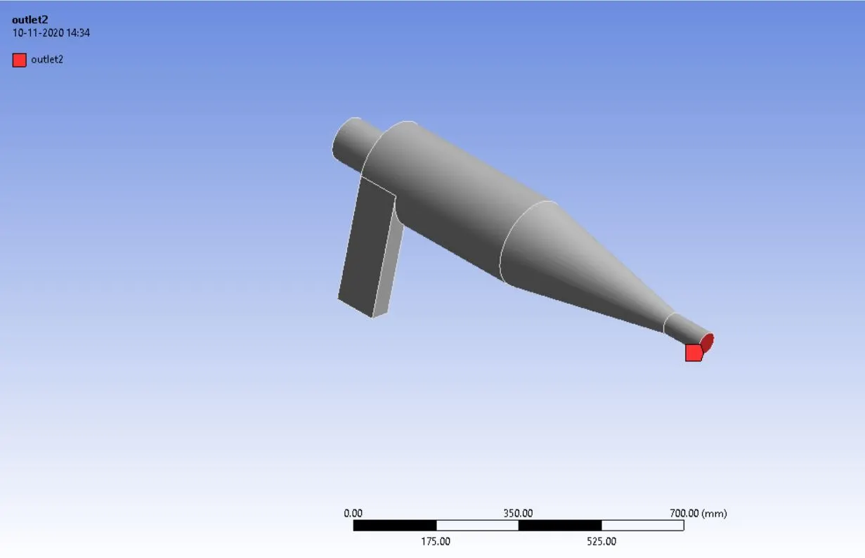
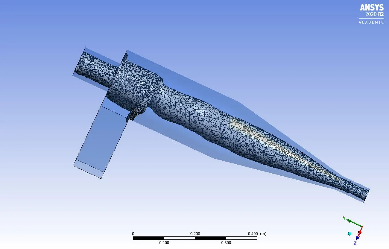
7. The mesh is successfully created.
8. 

Pre-processing physics setup:

1. Open the fluent console.
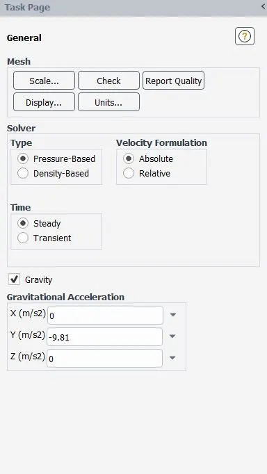
2. From the model tab choose pressure-based solver>> steady state simulation with gravity enabled in negative y direction.
3. 
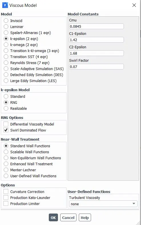
4. Select viscous model tab>> choose k-epsilon>> RNG >> swirl dominated>> scalable wall factor.
5. 
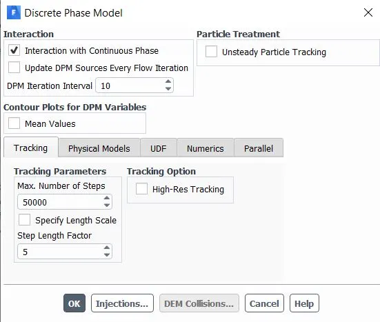
6. Select the discrete phase model >> choose the continuous phase mode.
7. 
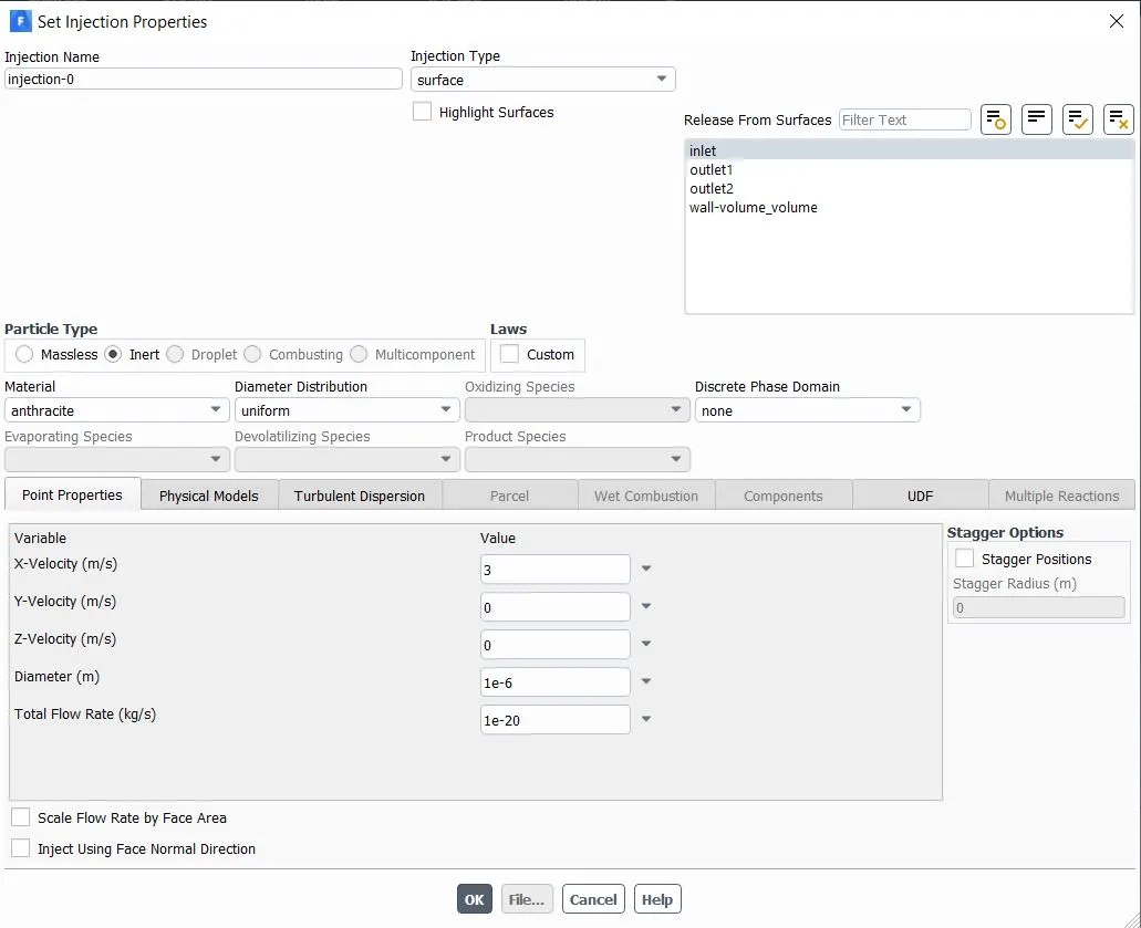
8. Select the injection tab option>> choose type as surface>> choose release from the inlet section.>> provide material as anthracite>> provide particle type as inert>> provide the particle diameter and x velocity flow of fluid according to different cases.
9. 
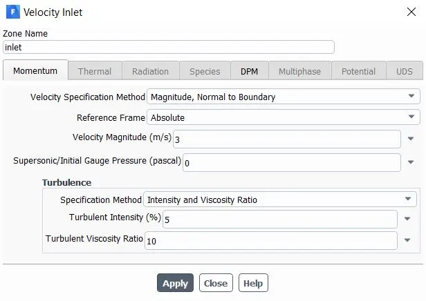
10. Now applying boundary condition for inlet choose velocity as per required case and select the type of DPM as reflect.
11. 
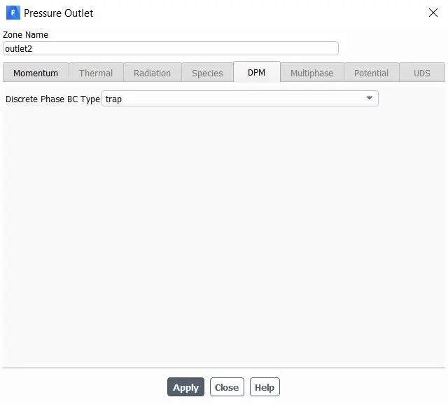
12. For outlet(top) choose as pressure outlet and select DPM as escape.
13. 
14. For outlet(bottom) choose as pressure outlet and select DPM as trap.
15. 
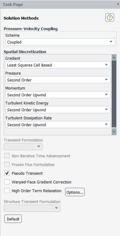
16. Go to solution tab and choose 2^nd order upwind scheme for the turbulent kinetic energy term.
17. 
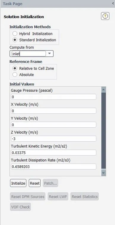
18. Choose standard initialization and compute from the inlet section.
19. 
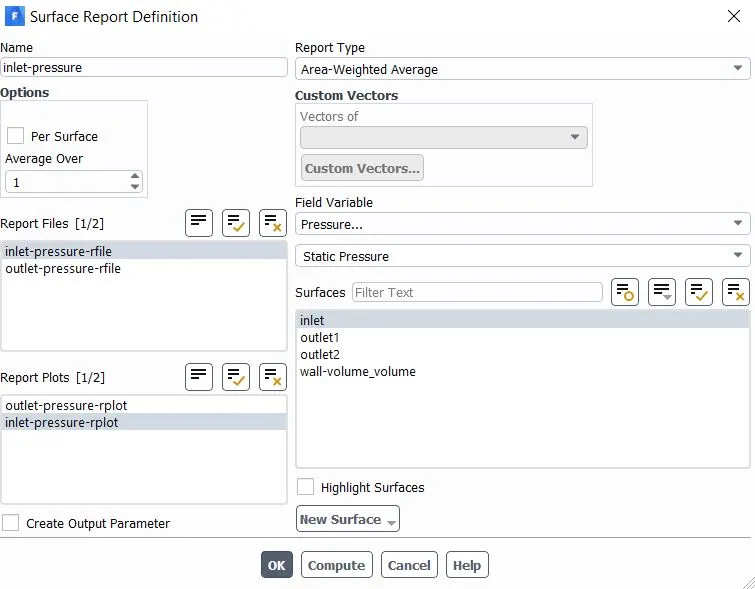
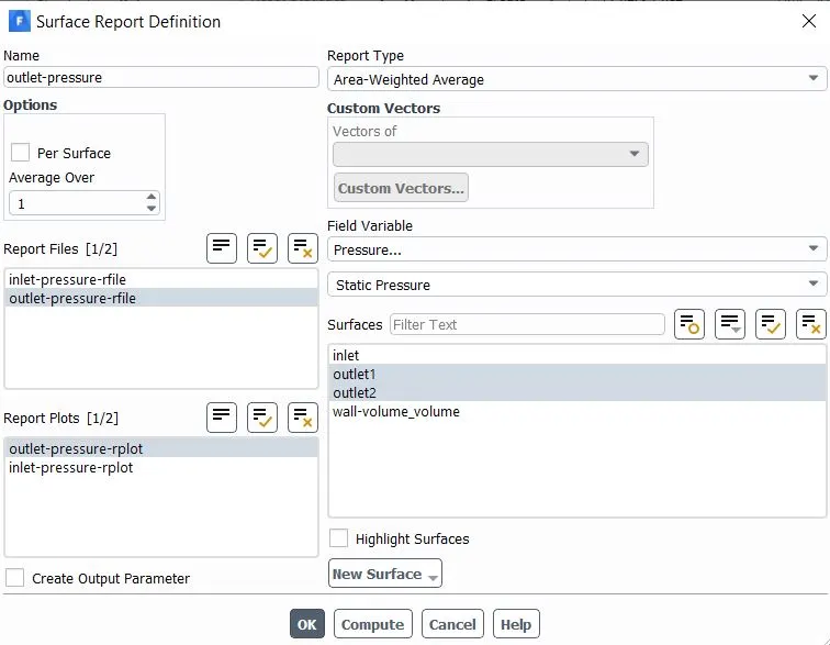
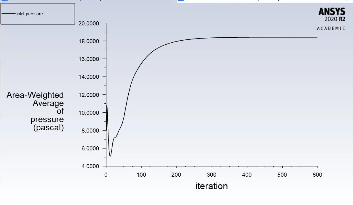
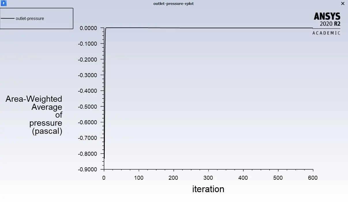
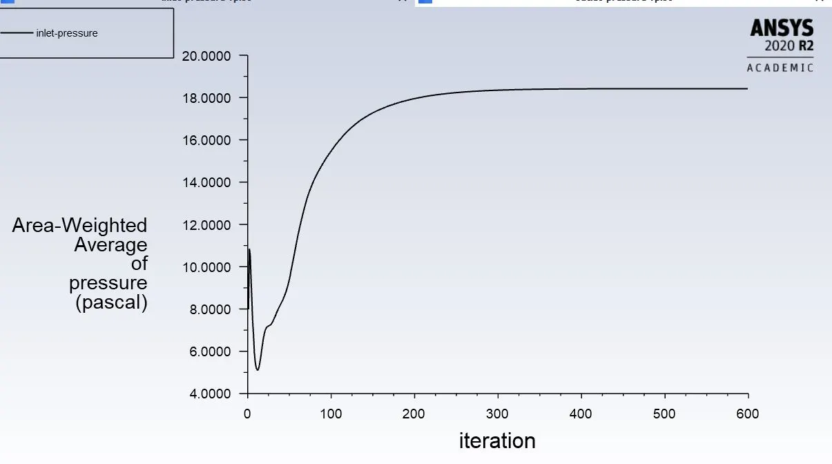
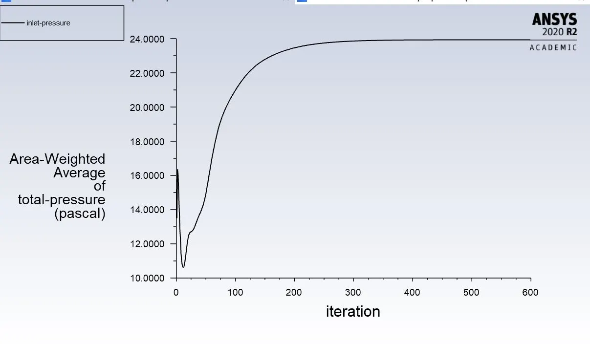
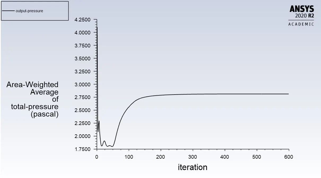
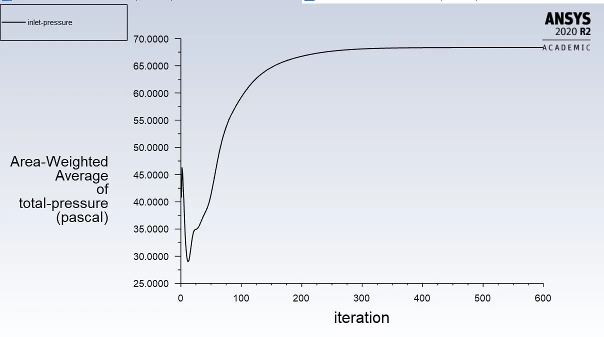
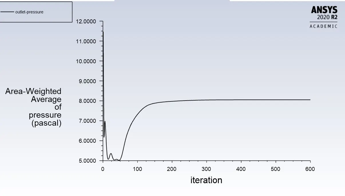
20. select parameters from the report definition as inlet and outlet pressure.
21. 
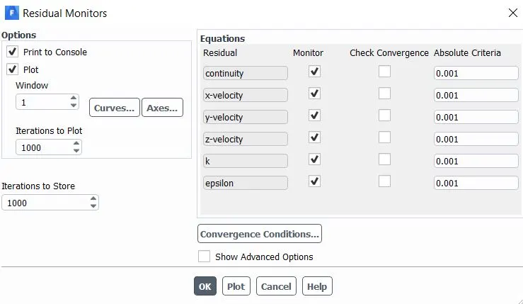
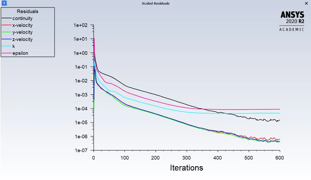
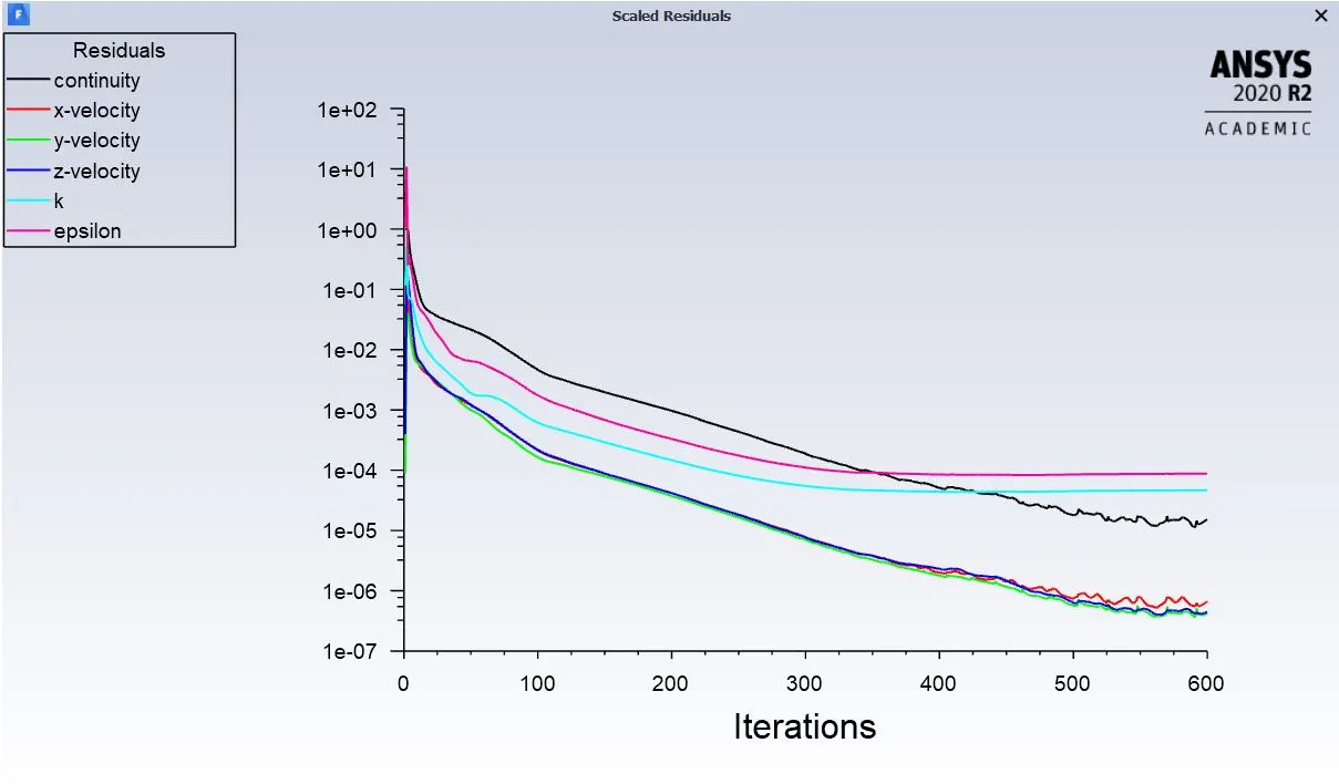
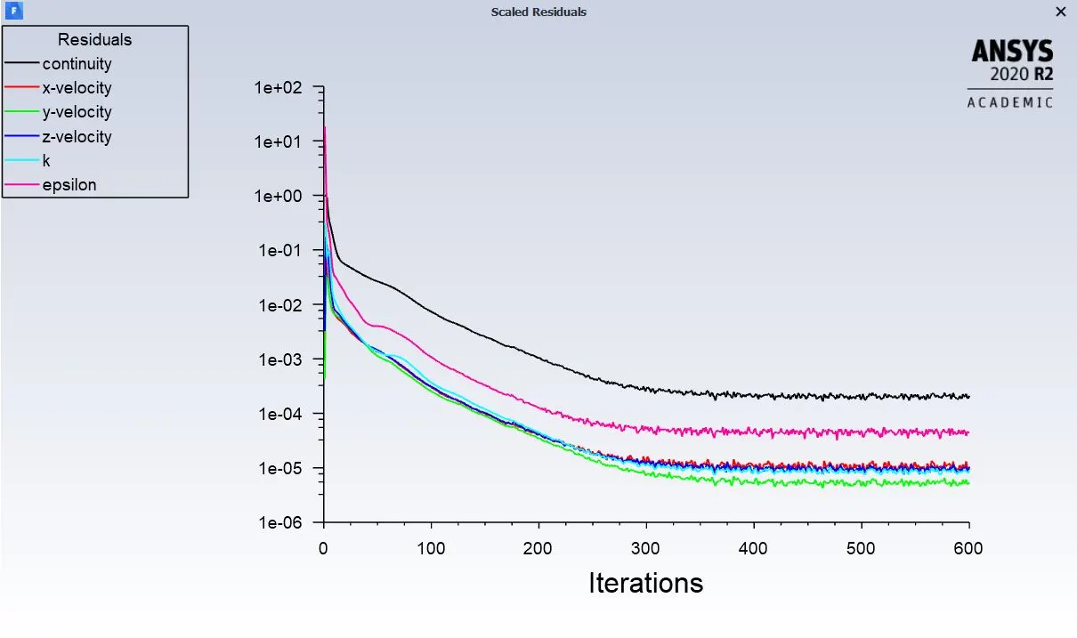
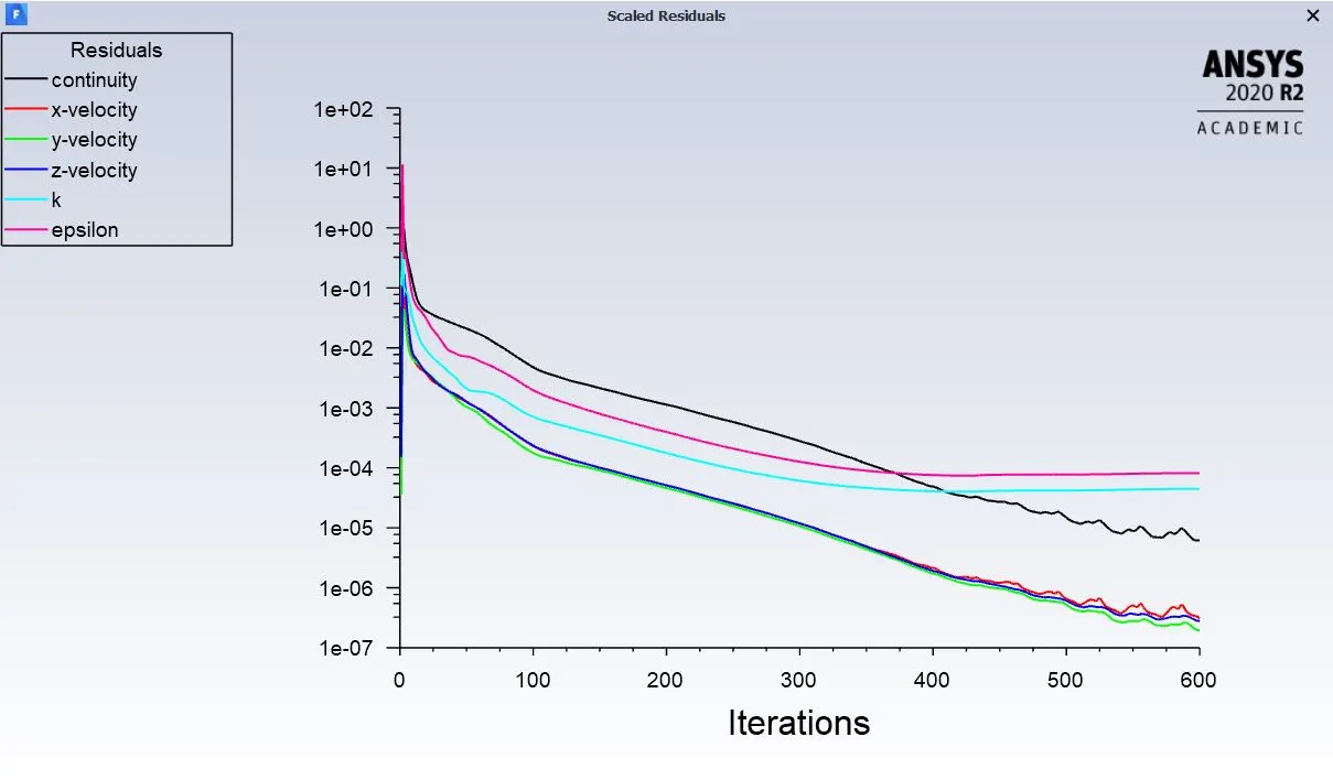
22. choose the convergence settings
23. 
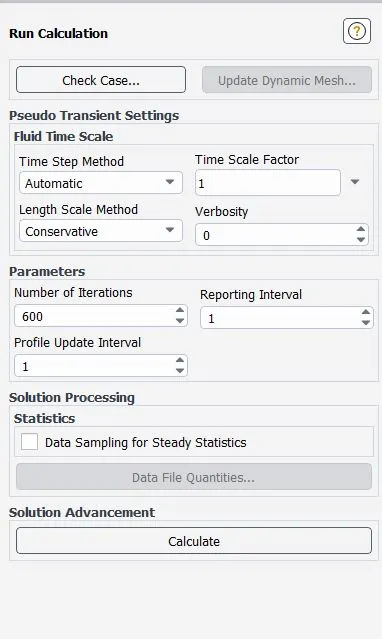
24. Provide the no of iterations and run the solver.
25. 

Part 1: To perform an analysis on the cyclone separator model by varying the particle diameter from 1-5micrometer, the separation efficiency in each case. Use the particle velocity as 3m/s in each cases.

Case1:

Particle diameter:1µm

Particle velocity: 3m/s

Nodes:22858

Elements:112026

Vortex strength:

Iteration to converge:

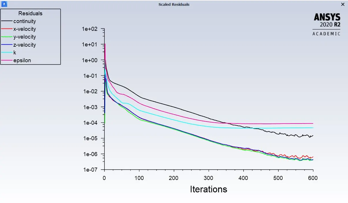
Particle tracked:120

Particle escaped:34

Particle trapped:18

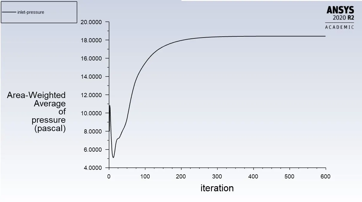
Inlet pressure:18.42002Pa

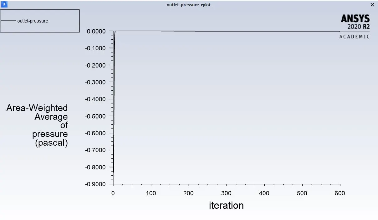
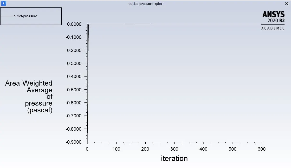
Outlet pressure:-0.0015531Pa

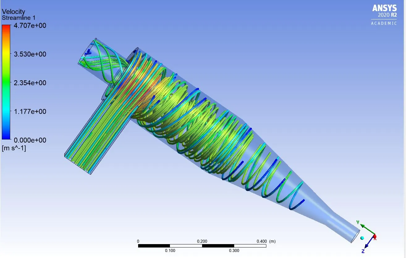
Velocity streamlines:

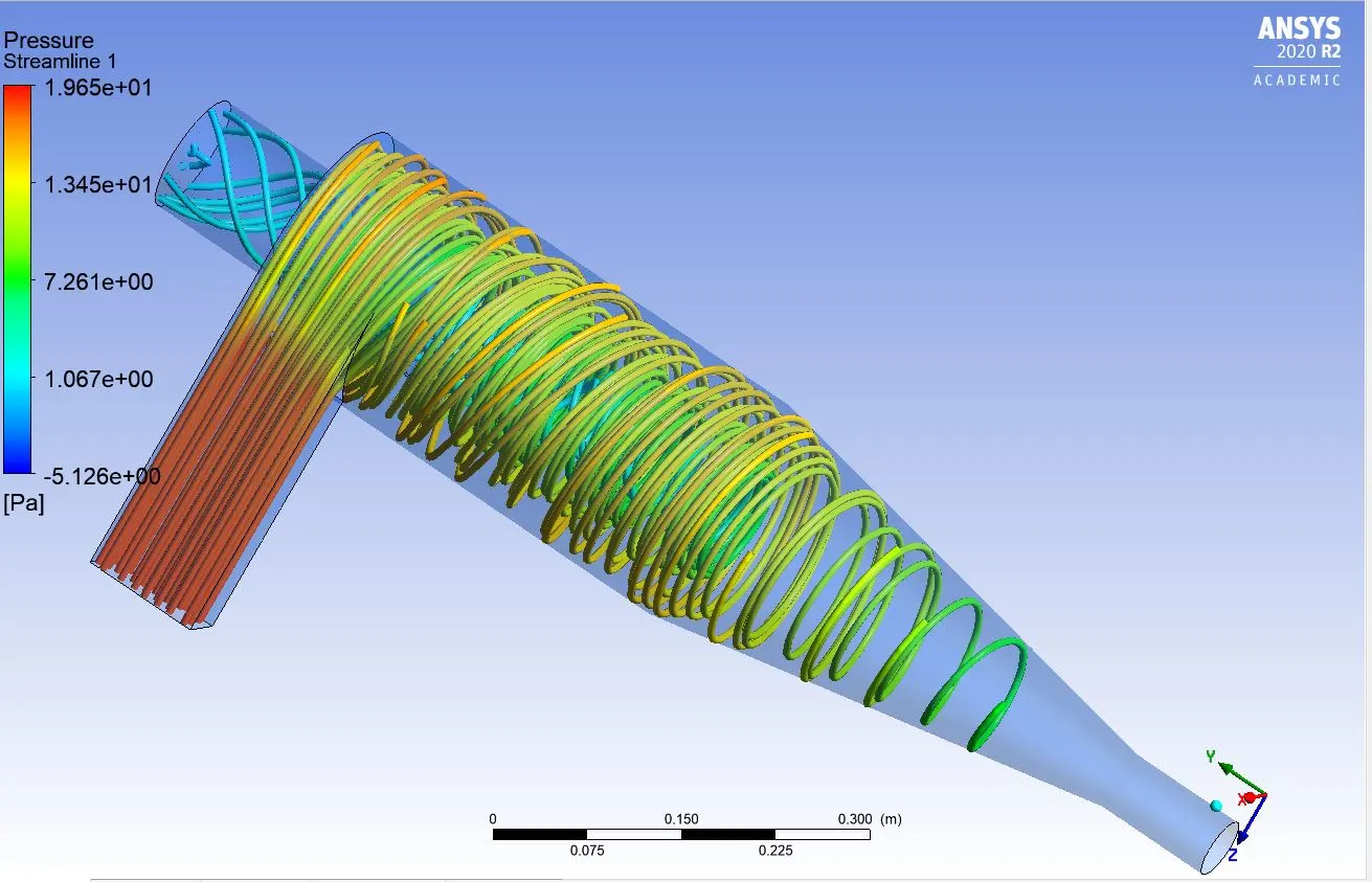
Pressure streamlines:

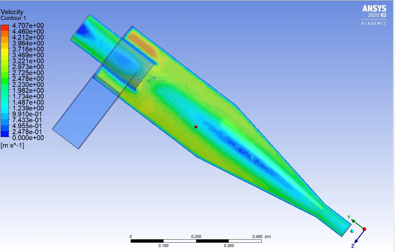
Velocity contour:

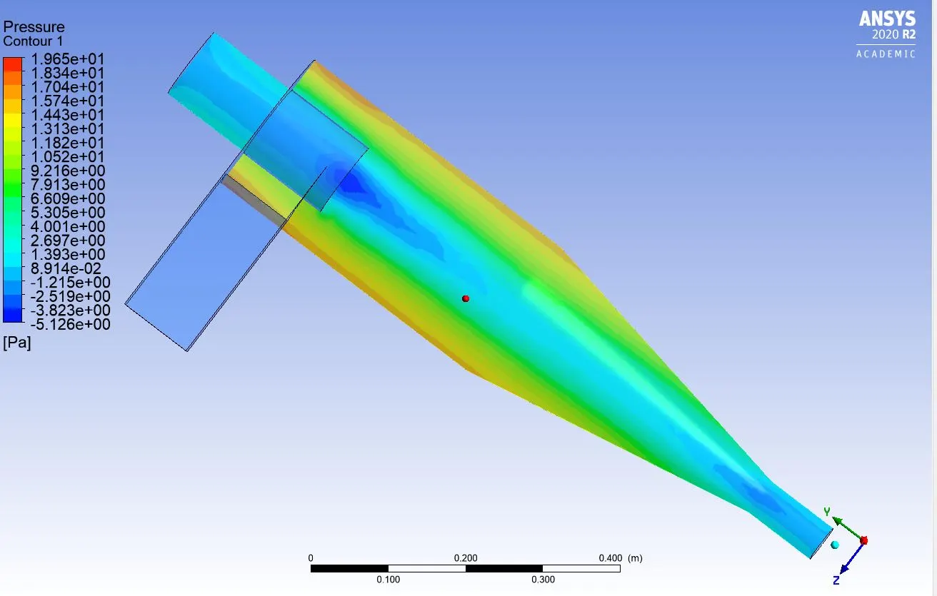
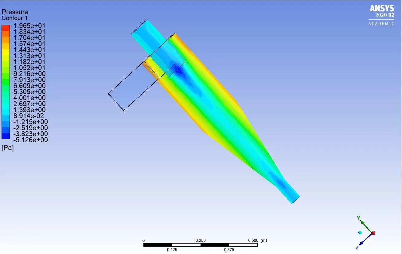
Pressure contour:

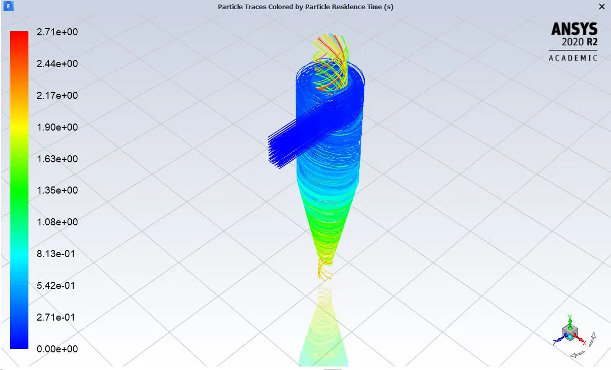
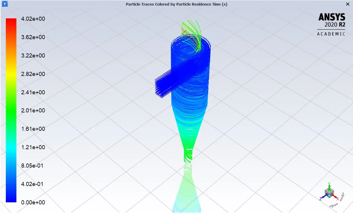
Particle track time:

Animation:

Velocity flow:

Pressure flow:

Computation of efficiency:

Efficiency=no of particles trapped/no of particles tracked=0.15

Case2:

Particle diameter:3µm

Particle velocity: 3m/s

Nodes:22858

Elements:112026

Vortex strength:

Iteration to converge:

Particle tracked:120

Particle escaped:21

Particle trapped:99

Inlet pressure:18.42004Pa

Outlet pressure:-0.0015531Pa

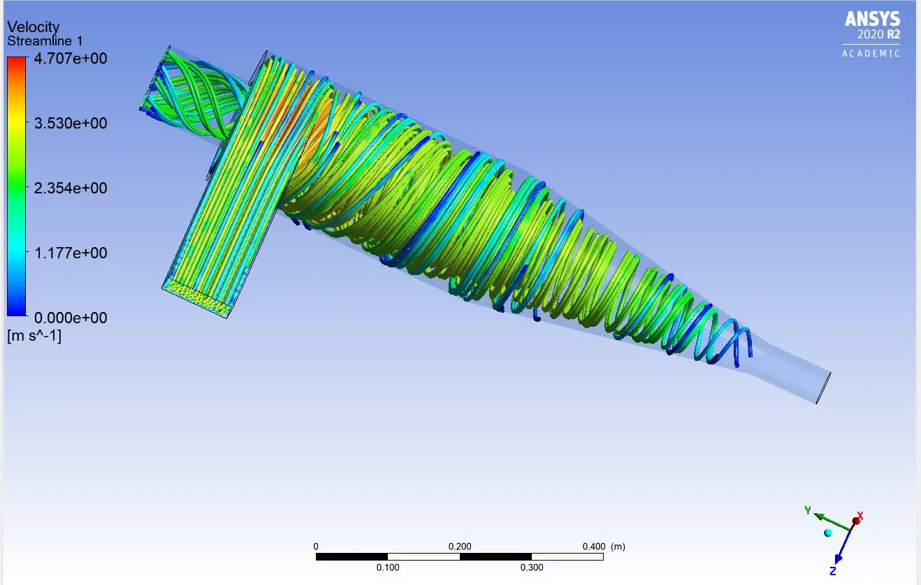
Velocity streamlines:

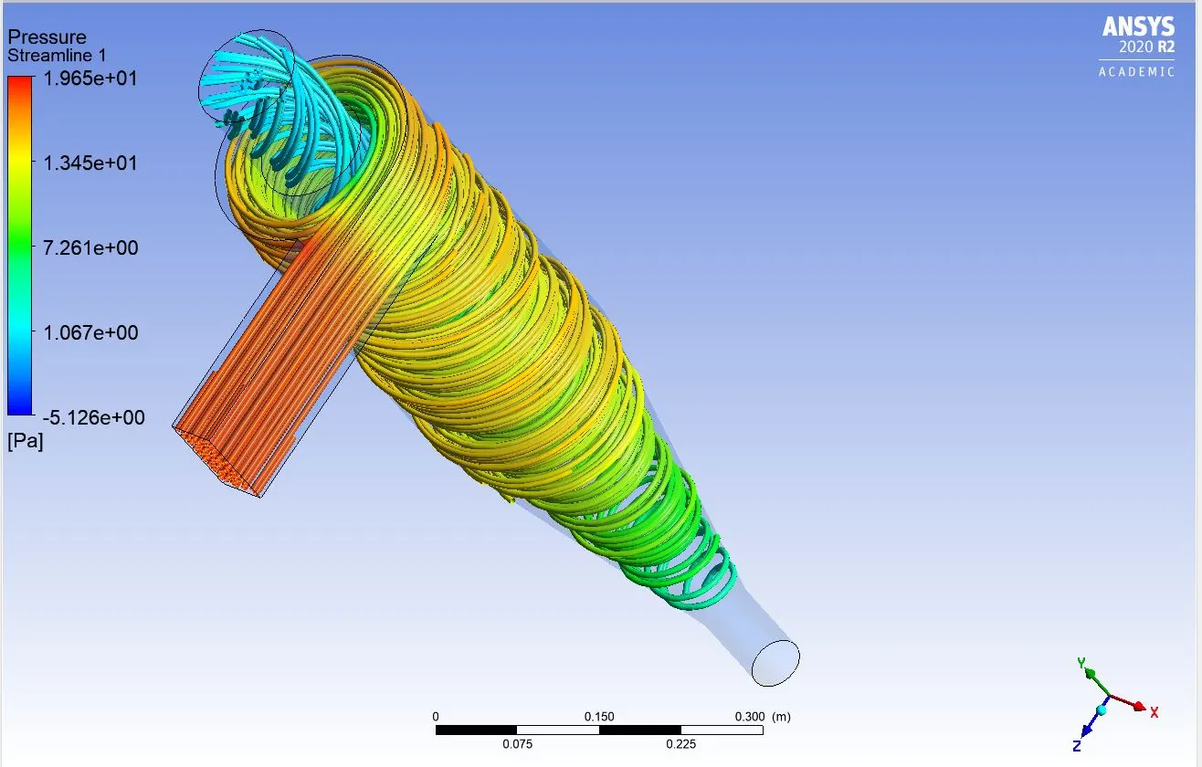
Pressure streamlines:

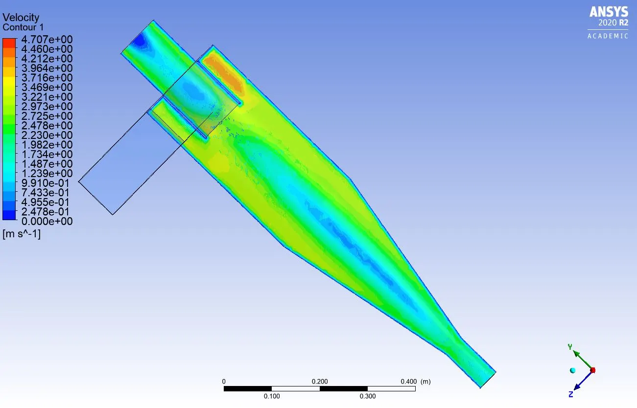
Velocity contour:

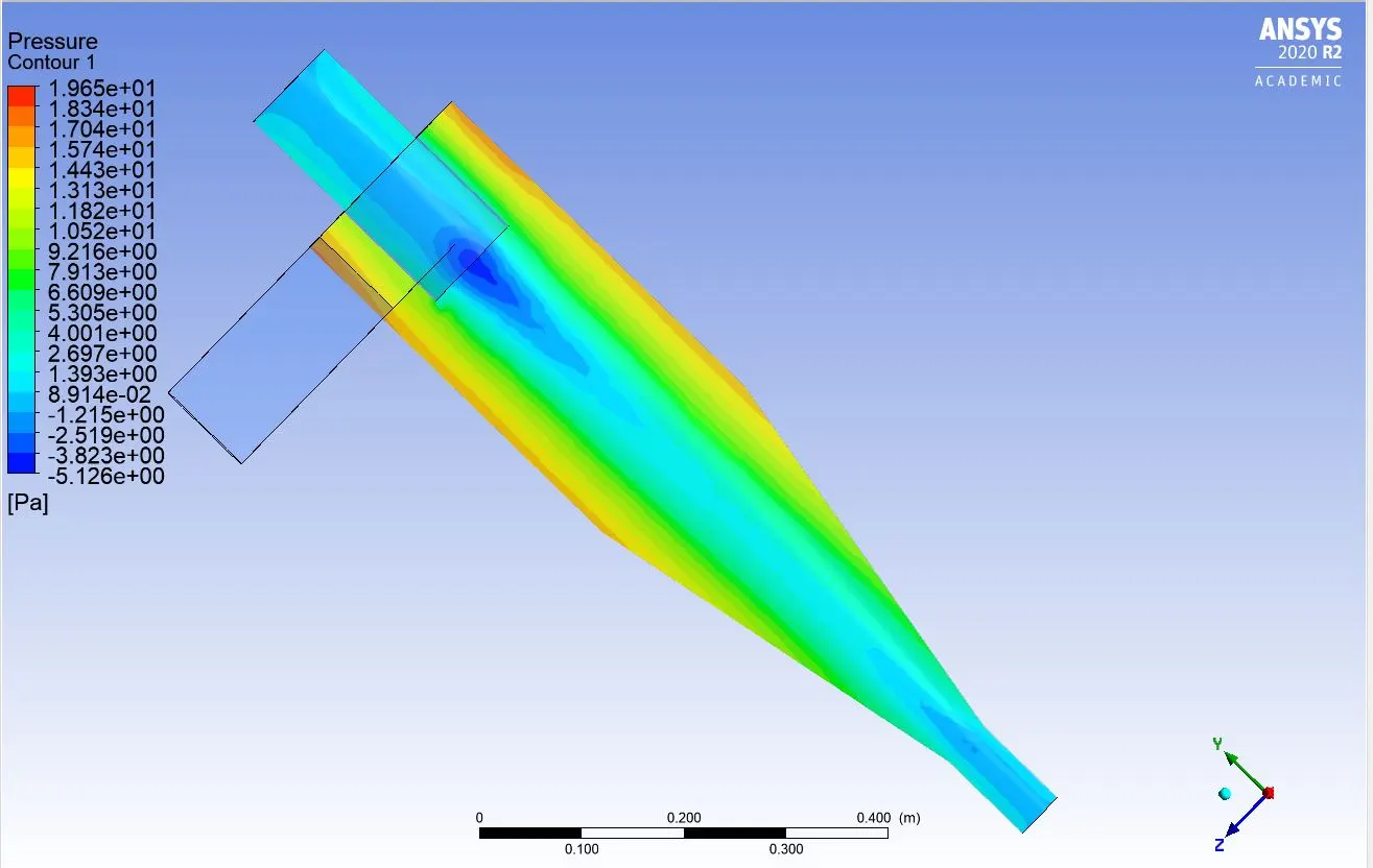
Pressure contour:

Particle track time:

Animation:

Velocity flow:

Pressure flow:

Computation of efficiency:

Efficiency=no of particles trapped/no of particles tracked=0.825

Case3:

Particle diameter:5µm

Particle velocity: 3m/s

Nodes:22858

Elements:112026

Vortex strength:

Iteration to converge:

Particle tracked:120

Particle escaped:0

Particle trapped:120

Inlet pressure:

Outlet pressure:

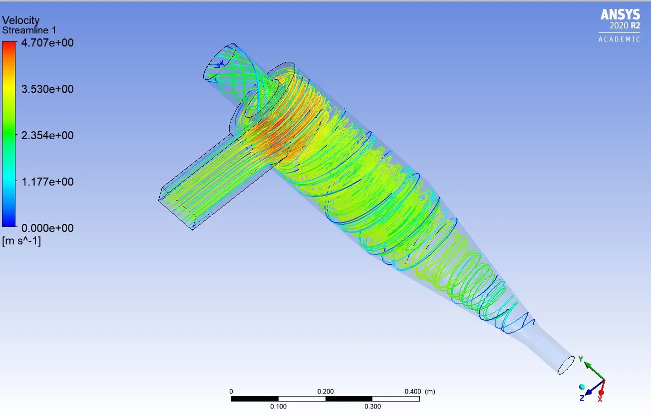
Velocity streamlines:

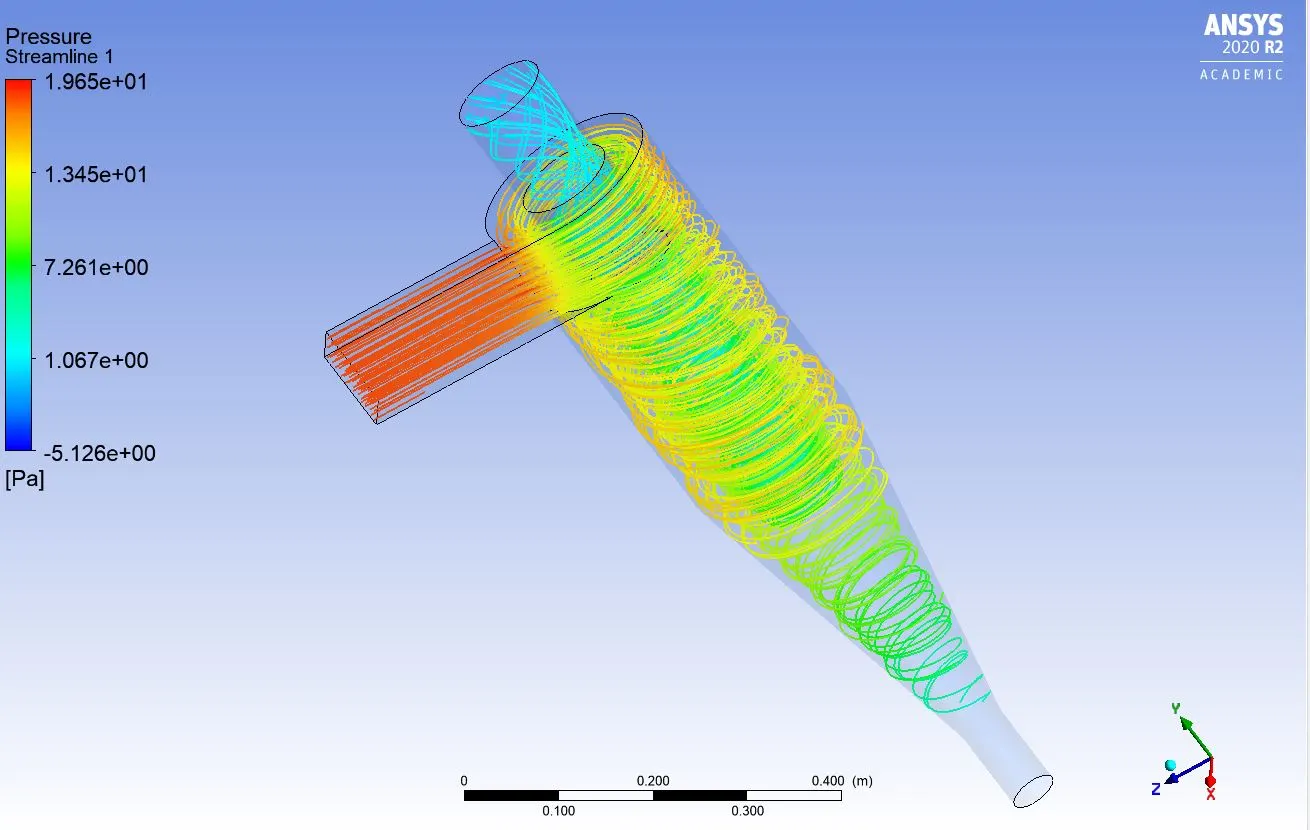
Pressure streamlines:

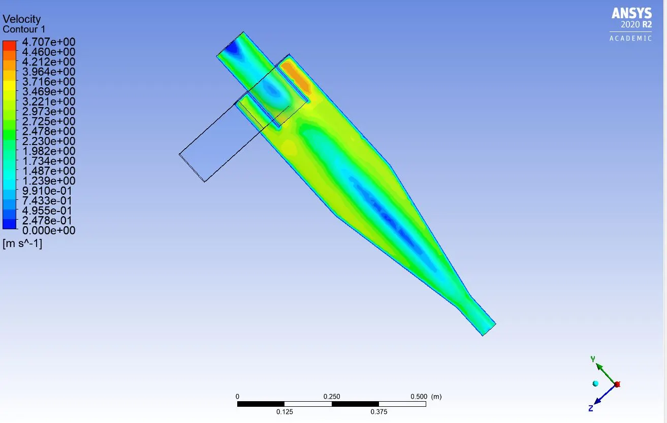
Velocity contour:

Pressure contour:

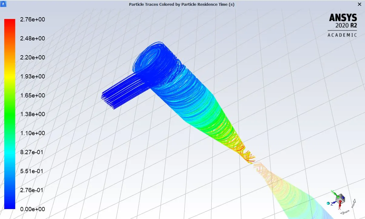
Particle track time:

Animation:

Velocity flow:

Pressure flow:

Computation of efficiency:

Efficiency=no of particles trapped/no of particles tracked=1.

Comparison of different cases from the above case studies:

Particle diameter	Pressure change (Pa)	Inlet mass flow	Outlet mass flow(top)	Outlet mass flow(bottom)	Efficiency
1 µm	18.4184	0.018375	0.014788	0.00358619	15%
3 µm	18.4184	0.018375	0.014788	0.00358619	82.5%
5 µm	18.4184	0.018375	0.014788	0.00358619	100%

Discussions:

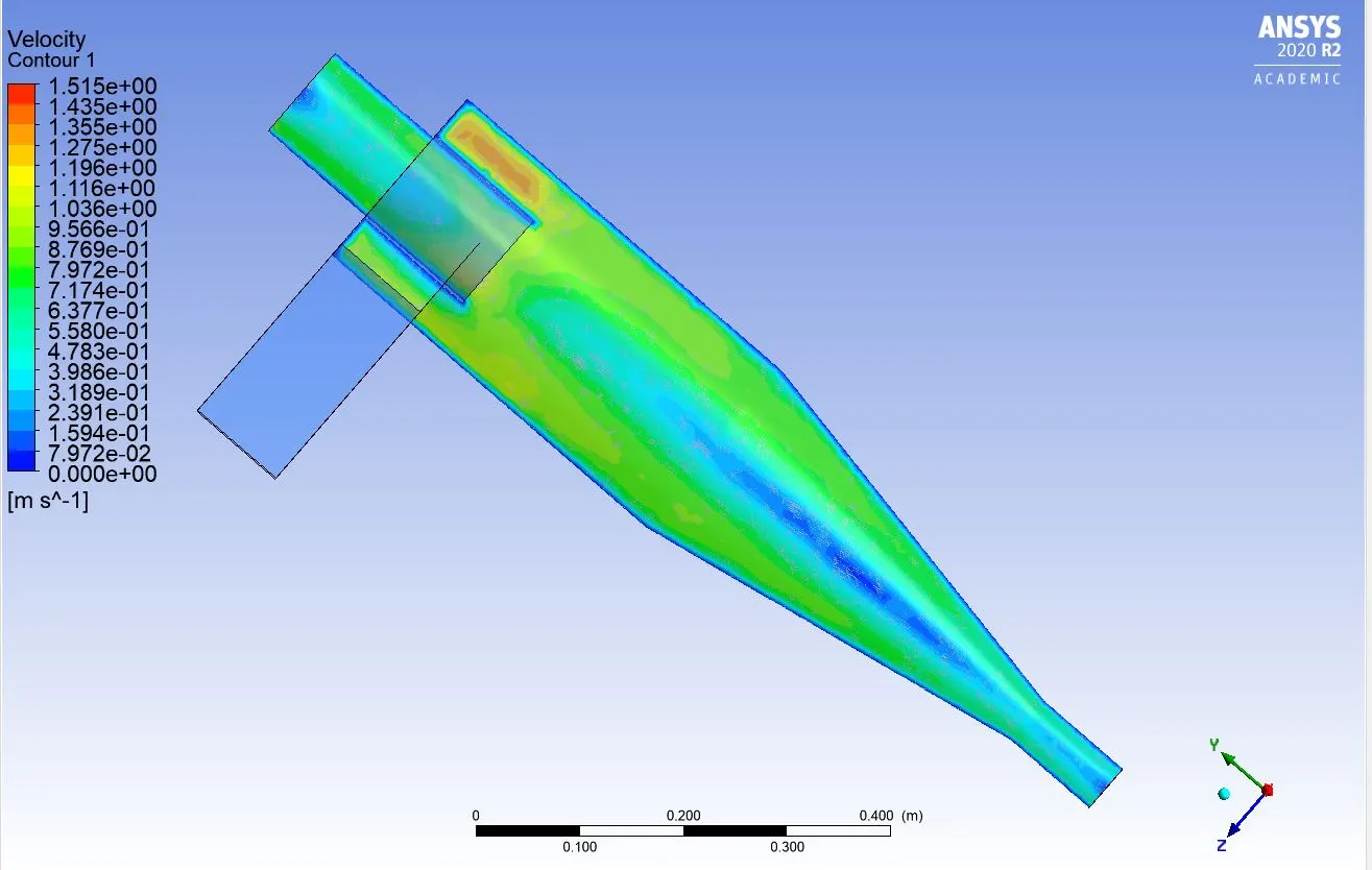
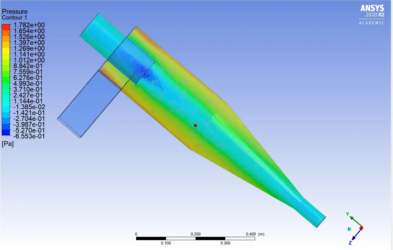
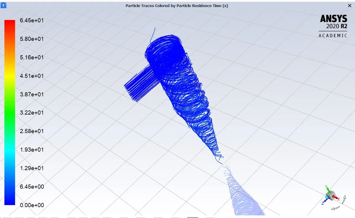
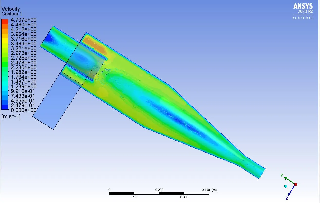
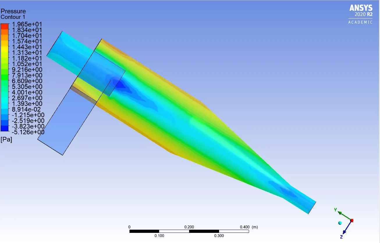
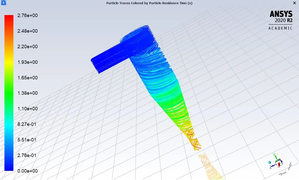
From the computation table we see that particle diameter has an influence in increasing the efficiency of cyclone separator model. Now, since the velocity of flow is kept constant, the pressure change also remains constant, the change in static pressure is also constant. the efficiency of the model depends upon the particle dia and the particle tracked data. The particle track time is seen to decrease from 5.06s to 2.71s, on varying the diameter from 1 µm to 5 µm, which demonstrates the time for settlement. The pressure contour region shows higher at the model wall and less at the outlet section, this predicts a constant mass flow rate at the outlet section. The efficiency overall depends upon the particle diameter as a function.

Part 2: To perform an analysis on a given cyclone separator model by varying the particle velocity from 1 m/sec to 5 m/sec and calculate the separation efficiency and pressure drop in each case. Discuss the results. [Use particle diameter size as 5 μm for all cases & keep flow velocity same as particle velocity]

Case1:

Particle diameter:5µm

Particle velocity: 1m/s

Nodes:22858

Elements:112026

Vortex strength:

Iteration to converge:

Particle tracked:120

Particle escaped:2

Particle trapped:5

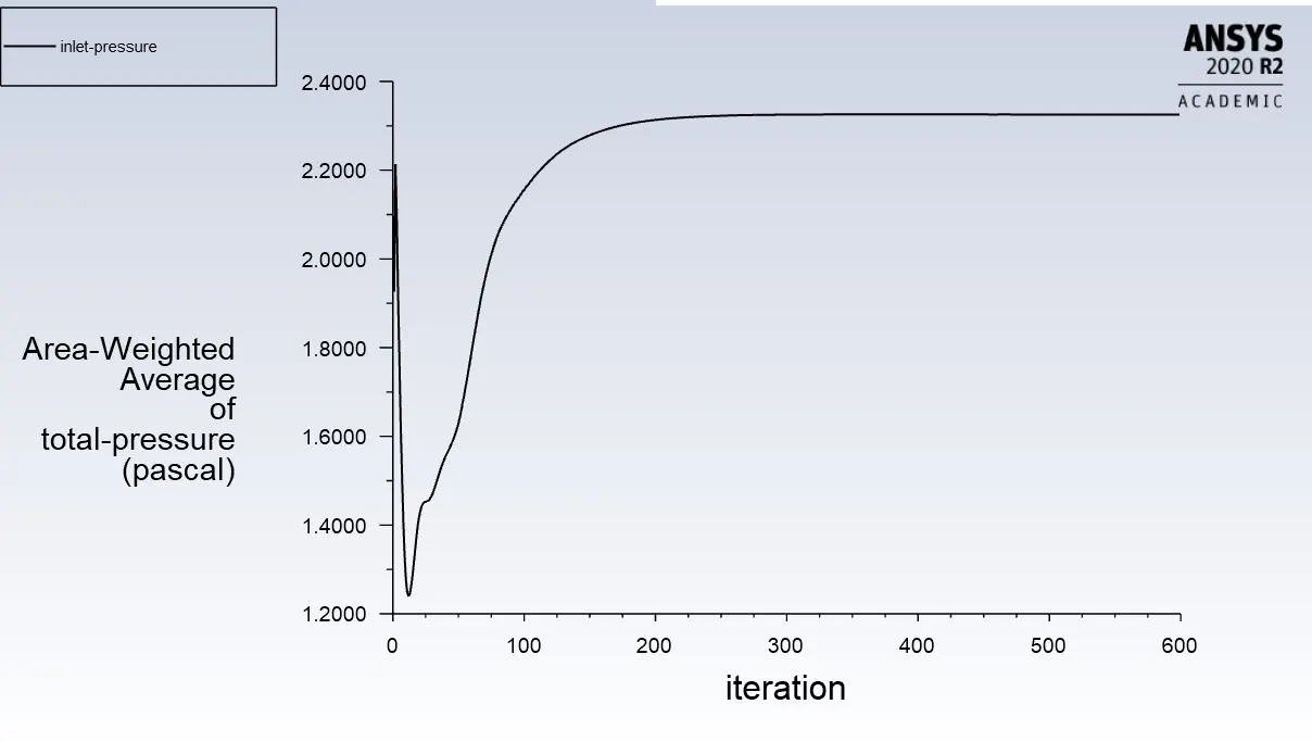
Inlet pressure:2.325527Pa

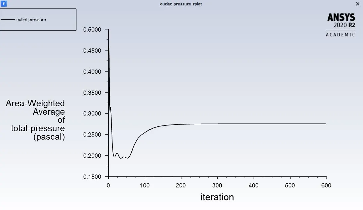
Outlet pressure:0.275314Pa

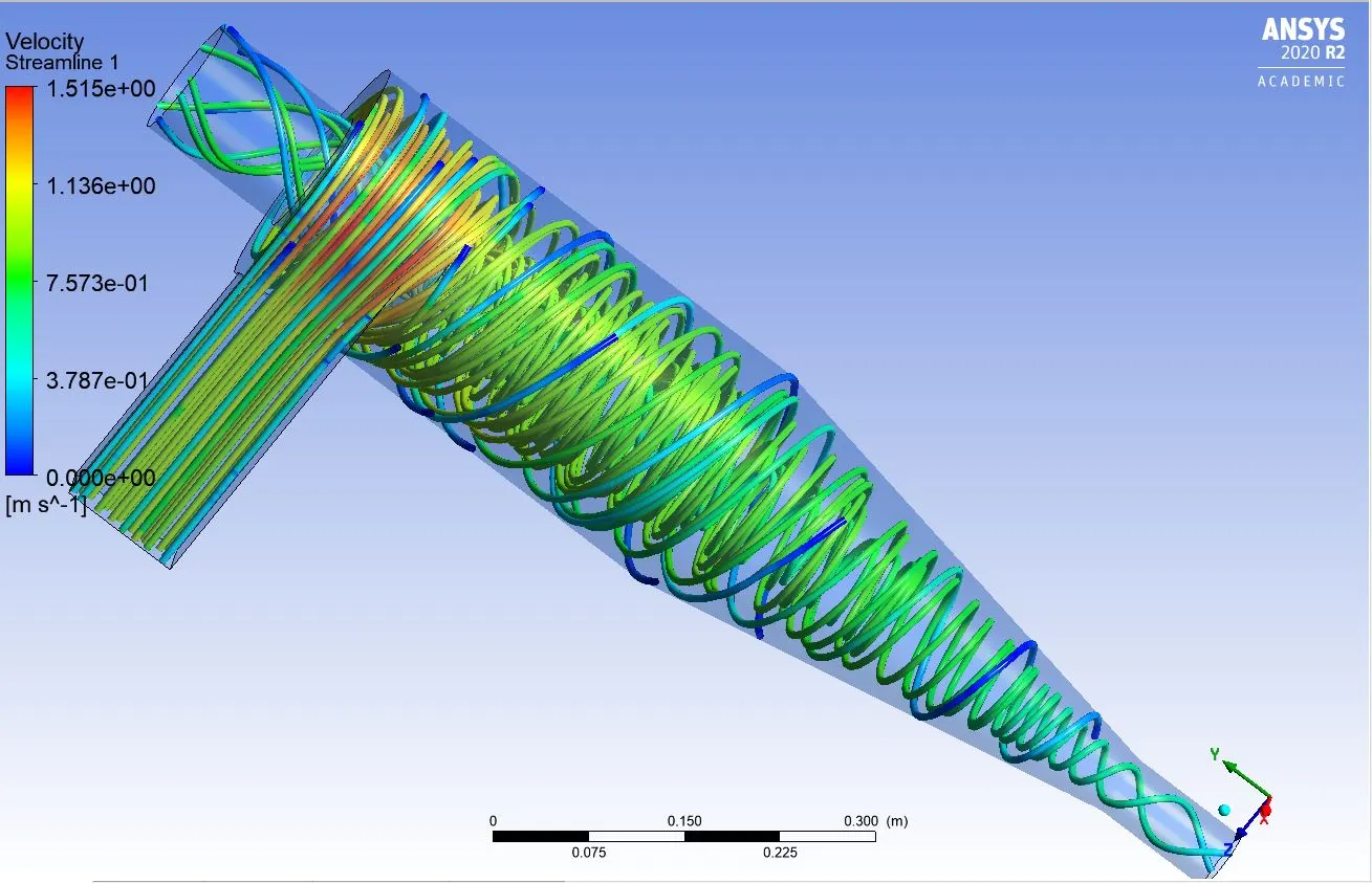
Velocity streamlines:

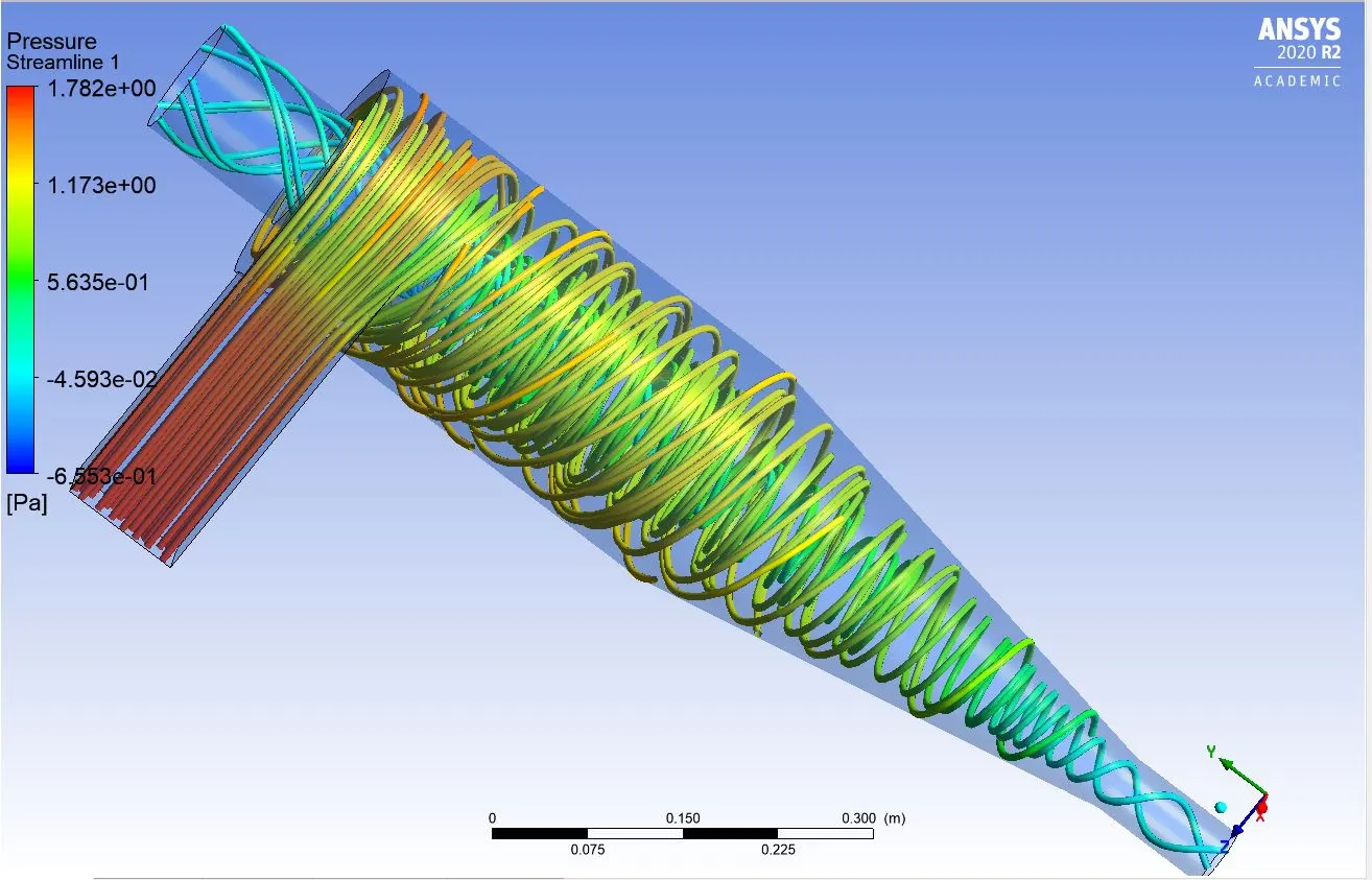
Pressure streamlines:

Velocity contour:

Pressure contour:

Particle track time:

Animation:

Velocity flow:

Pressure flow:

Computation of efficiency:

Efficiency=no of particles trapped/no of particles tracked=0.0416.

Case2:

Particle diameter:5µm

Particle velocity: 3m/s

Nodes:22858

Elements:112026

Vortex strength:

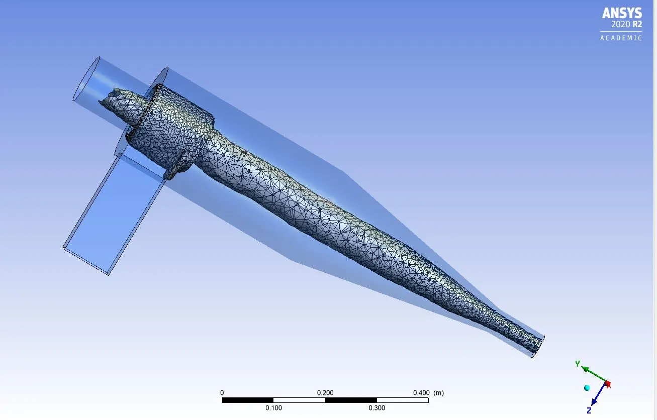
Iteration to converge:

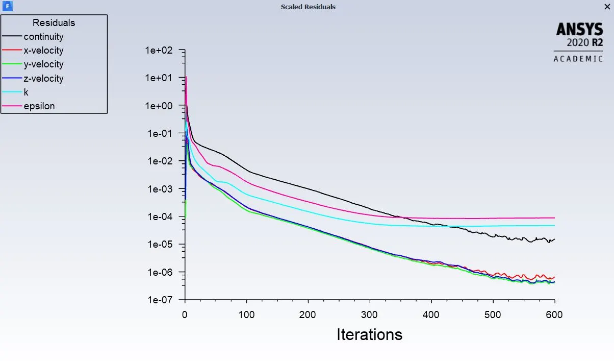
Particle tracked:120

Particle escaped:6

Particle trapped:114

Inlet pressure:23.92988Pa

Outlet pressure:2.8125Pa

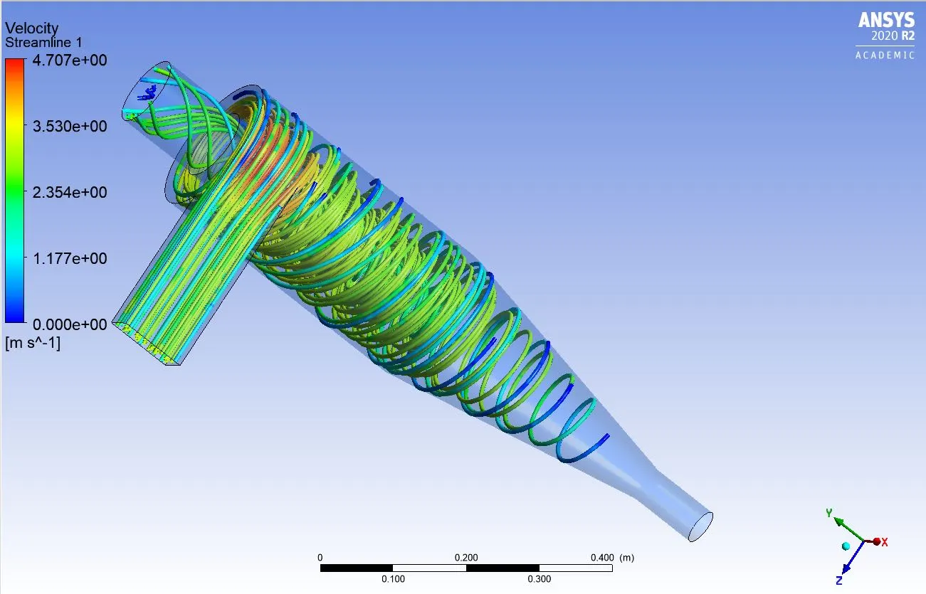
Velocity streamlines:

Pressure streamlines:

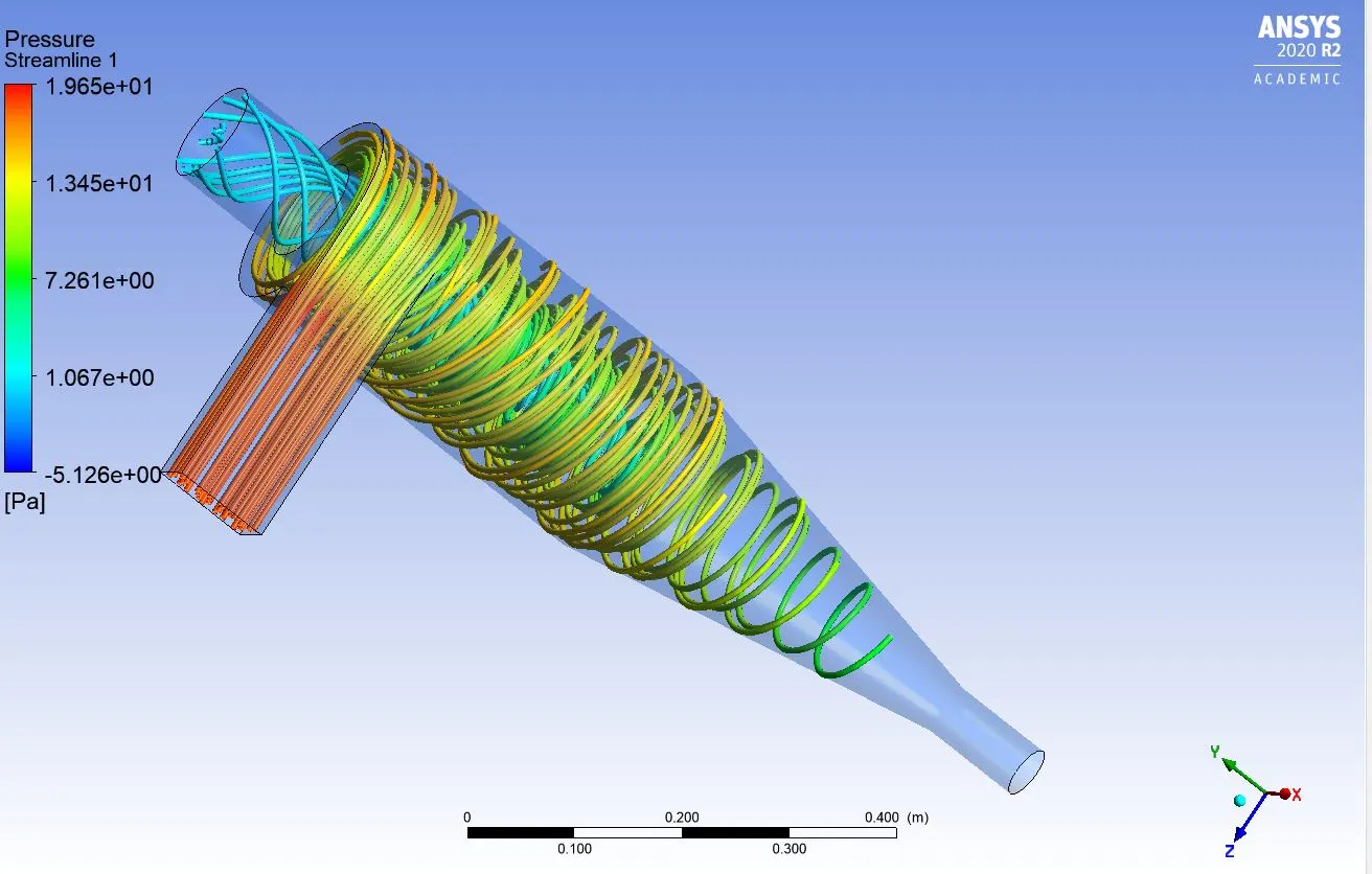
Velocity contour:

Pressure contour:

Particle track time:

Animation:

Velocity flow:

Pressure flow:

Computation of efficiency:

Efficiency=no of particles trapped/no of particles tracked=0.95

Case3:

Particle diameter:5µm

Particle velocity: 5m/s

Nodes:22858

Elements:112026

Vortex strength:

Iteration to converge:

Particle tracked:120

Particle escaped:0

Particle trapped:120

Inlet pressure:68.346806Pa

Outlet pressure:8.0396Pa

Velocity streamlines:

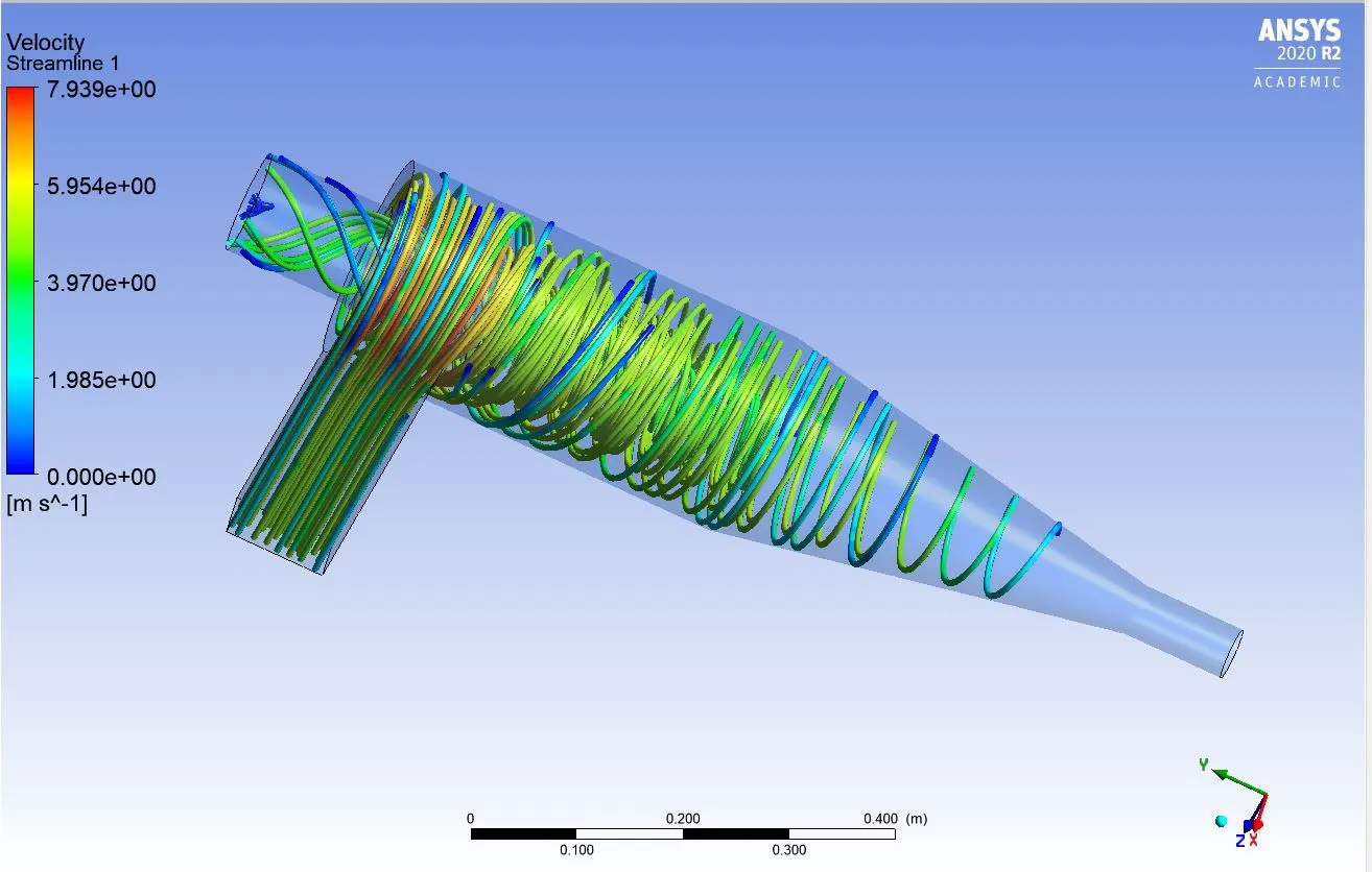
Pressure streamlines:

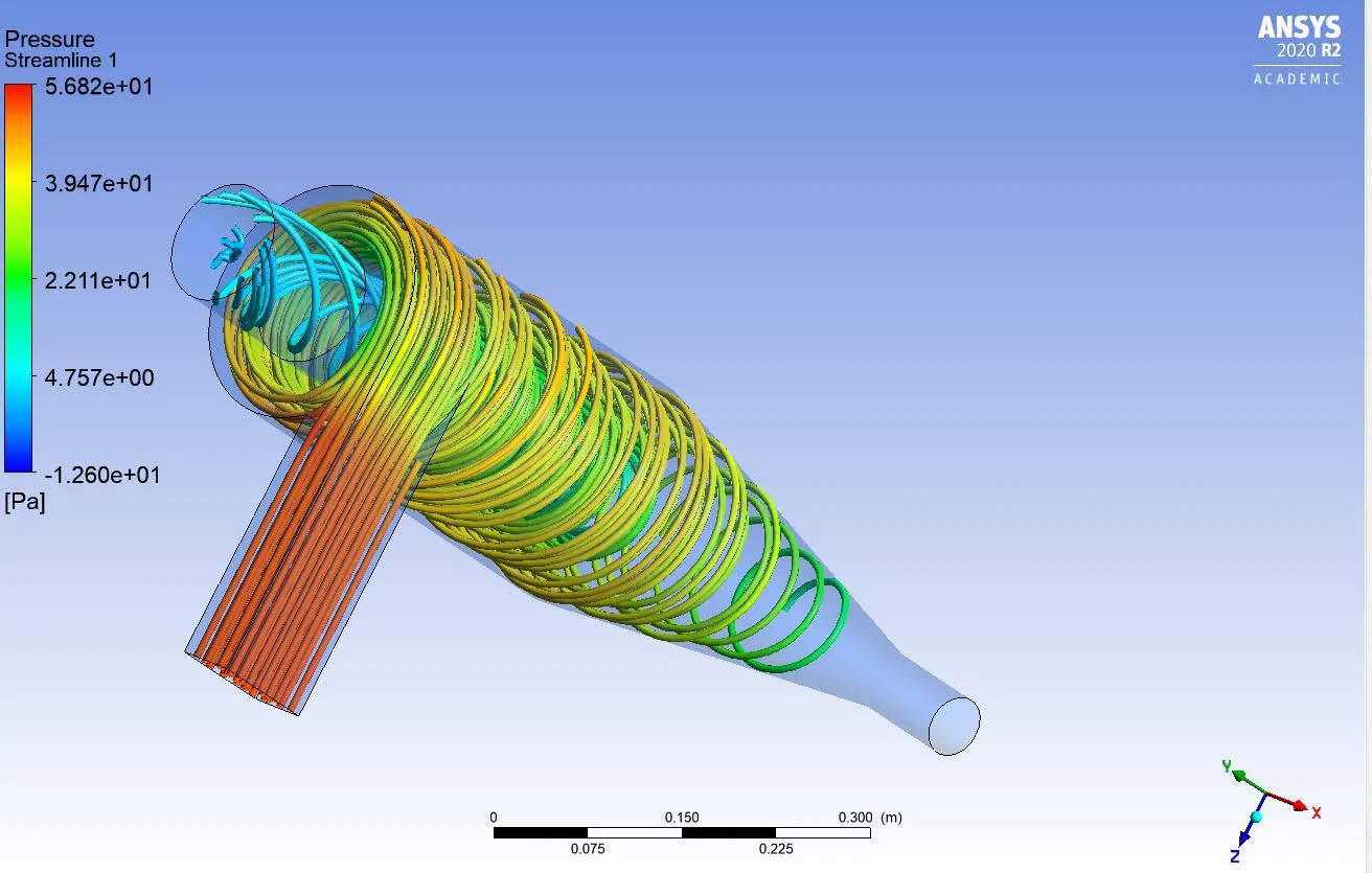
Velocity contour:

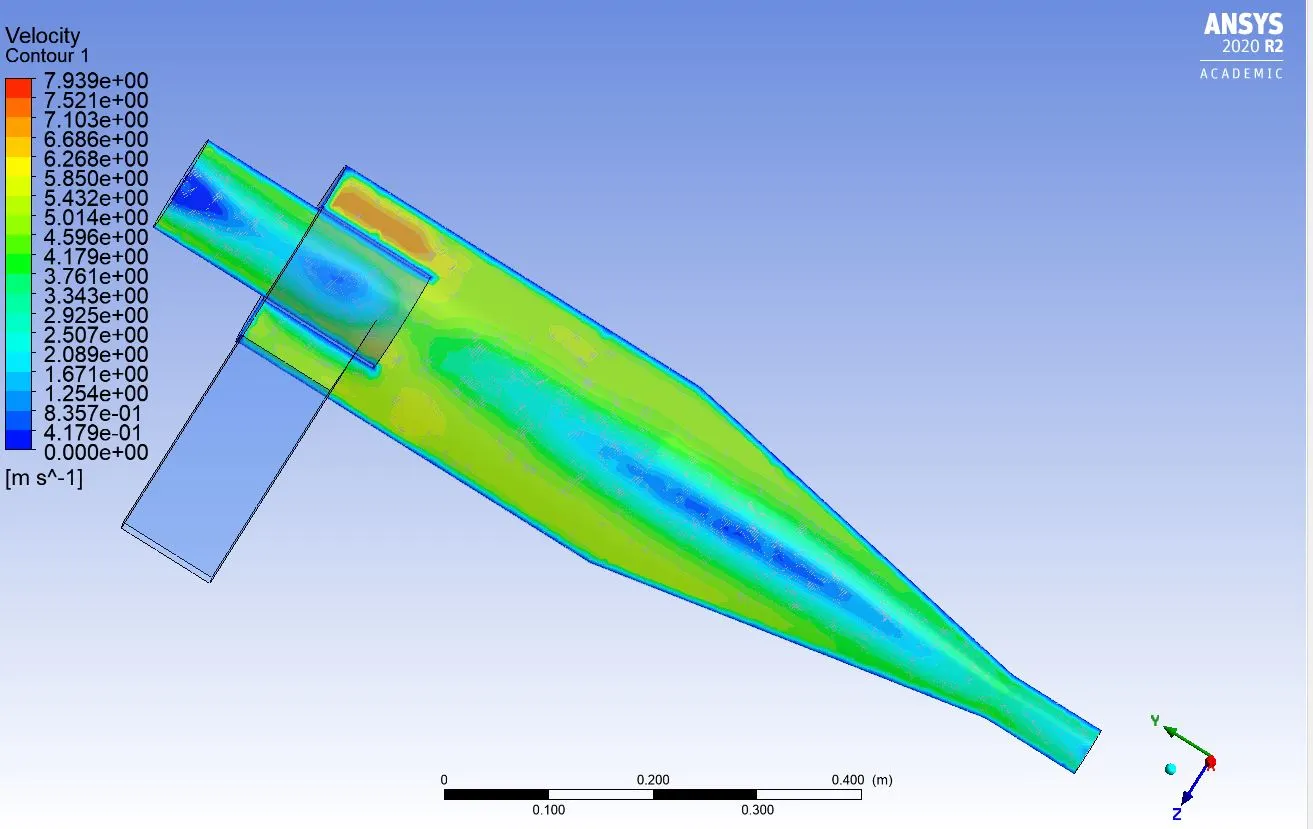
Pressure contour:

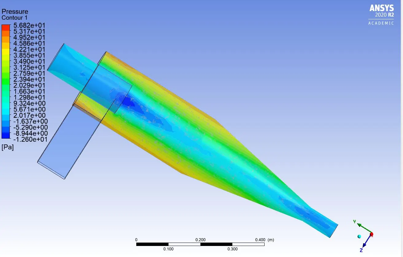
Particle track time:

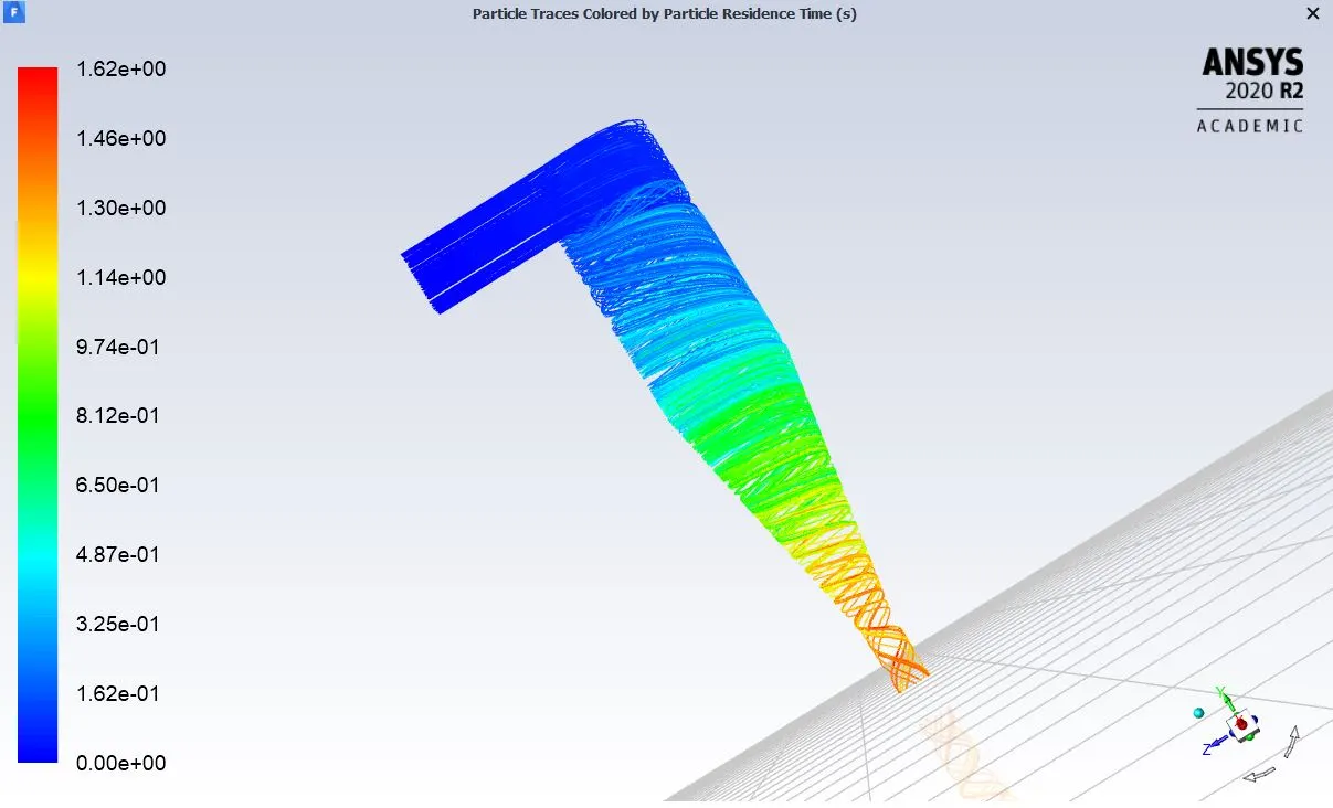
Animation:

Velocity flow:

Pressure flow:

Computation of efficiency:

Efficiency=no of particles trapped/no of particles tracked=1

Comparison of different cases from the above case studies:

Velocity change (m/s)	Pressure change (Pa)	Inlet mass flow	Outlet mass flow(top)	Outlet mass flow(bottom)	Efficiency
1	2.05022	0.00628	0.00515117	0.0009728	4%
3	21.11738	0.018375	0.014788	0.00358619	95%
5	60.29484	0.030623	0.024674	0.00595065	100%

Discussions:

From the case 2 data set we see that the efficiency of the model depends upon the particle velocity. With a fixed particle dia the velocity is varied in three cases, where the change in total pressure is seen to increase, even the mass flow rate changes as a function of velocity change. The efficiency is higher at particle velocity of 5m/s. the particle track time also indicates less time with higher particle velocity, making the particles settle down faster and also increasing the efficiency of the model. Eventually the efficiency factor over here solely depends upon the velocity change.

Conclusions:

1. The cyclone separator efficiency has been achieved higher successfully in both the cases, but considering the change in velocity factor is more predominant in increasing the efficiency at a faster rate.
2. The maximum velocity of 7.939m/s is achieved for particle velocity of 5m/s and minimum of 1.37m/s is achieved for velocity factor of1m/s.
3. The mass flow rate appreciably increases with the total pressure change with velocity variations.
4. In conclusion the variation of particle velocity can be more optimal in increasing the design efficiency.