Week 8: Literature review - RANS derivation and analysis
Turbulence:
In fluid dynamics, turbulence or turbulent flow is fluid motion characterized by chaotic changes in pressure and flow velocity. It is in contrast to a laminar flow, which occurs when a fluid flows in parallel layers, with no disruption between those layers.
Turbulence is commonly observed in everyday phenomena such as surf, fast flowing rivers, billowing storm clouds, or smoke from a chimney, and most fluid flows occurring in nature or created in engineering applications are turbulent. Turbulence is caused by excessive kinetic energy in parts of a fluid flow, which overcomes the damping effect of the fluid's viscosity. For this reason turbulence is commonly realized in low viscosity fluids. In general terms, in turbulent flow, unsteady vortices appear of many sizes which interact with each other, consequently drag due to friction effects increases. This increases the energy needed to pump fluid through a pipe.
Turbulence modelling:
Turbulence modeling is the construction and use of a mathematical model to predict the effects of turbulence. Turbulent flows are commonplace in most real life scenarios, including the flow of blood through the cardiovascular system, the airflow over an aircraft wing, the re-entry of space vehicles, besides others. In spite of decades of research, there is no analytical theory to predict the evolution of these turbulent flows. The equations governing turbulent flows can only be solved directly for simple cases of flow. For most real life turbulent flows, CFD simulations use turbulent models to predict the evolution of turbulence. These turbulence models are simplified constitutive equations that predict the statistical evolution of turbulent flows.
Turbulence model classification:
The following is a brief overview of commonly employed models in modern engineering applications.
Spalart–Allmaras (S–A)
The Spalart–Allmaras model is a one-equation model that solves a modelled transport equation for the kinematic eddy turbulent viscosity. The Spalart–Allmaras model was designed specifically for aerospace applications involving wall-bounded flows and has been shown to give good results for boundary layers subjected to adverse pressure gradients. It is also gaining popularity in turbomachinery applications.
k–ε (k–epsilon)
K-epsilon (k-ε) turbulence model is the most common model used in computational fluid dynamics (CFD) to simulate mean flow characteristics for turbulent flow conditions. It is a two-equation model which gives a general description of turbulence by means of two transport equations (PDEs). The original impetus for the K-epsilon model was to improve the mixing-length model, as well as to find an alternative to algebraically prescribing turbulent length scales in moderate to high complexity flows.
k–ω (k–omega)
In computational fluid dynamics, the k–omega (k–ω) turbulence model is a common two-equation turbulence model that is used as a closure for the Reynolds-averaged Navier–Stokes equations (RANS equations). The model attempts to predict turbulence by two partial differential equations for two variables, k and ω, with the first variable being the turbulence kinetic energy (k) while the second (ω) is the specific rate of dissipation (of the turbulence kinetic energy k into internal thermal energy).
SST (Menter’s Shear Stress Transport)
SST (Menter's shear stress transport) turbulence model is a widely used and robust two-equation eddy-viscosity turbulence model used in computational fluid dynamics. The model combines the k-omega turbulence model and K-epsilon turbulence model such that the k-omega is used in the inner region of the boundary layer and switches to the k-epsilon in the free shear flow.
Reynolds stress equation model
The Reynolds stress equation model (RSM), also referred to as second moment closure model, is the most complete classical turbulence modelling approach. Popular eddy-viscosity based models like the k–ε (k–epsilon) model and the k–ω (k–omega) models have significant shortcomings in complex engineering flows. This arises due to the use of the eddy-viscosity hypothesis in their formulation. For instance, in flows with high degrees of anisotropy, significant streamline curvature, flow separation, zones of recirculating flow or flows influenced by rotational effects, the performance of such models is unsatisfactory. In such flows, Reynolds stress equation models offer much better accuracy.
Eddy viscosity based closures cannot account for the return to isotropy of turbulence, observed in decaying turbulent flows. Eddy-viscosity based models cannot replicate the behaviour of turbulent flows in the Rapid Distortion limit, where the turbulent flow essentially behaves like an elastic medium.
Various forms of Vavier Stokes equation
continuity equation
`(∂u)/(∂x)+(∂v)/(∂y)=0`
Momentum equation
`ρ((∂u)/(∂t)+u (∂u)/(∂x)+v (∂v)/(∂y))=-(∂P)/(∂x)+μ (∂^2 u)/(∂x^2 )`
Energy equation:
`ρc((∂T)/(∂t)+u (∂T)/(∂x)+v (∂T)/(∂y))=k(∂^2 T)/(∂x^2 )+μ ((∂ u)/(∂x ))^2`
To apply the Reynolds decomposition and came up with Reynolds stress
The components of terms are distributed in average and fluctuating parts
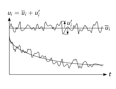
`u=u ̅+u^'`
`v=v ̅+v'`
`w=w ̅+w^'`
`p=p ̅+p'`
Chosen averaging method takes the mean value at a fixed place at a space domain and averaging it over a time span for the mean values to be large enough to be independent of
`u ̅=(1 )/(∆T) ∫_(T0)^(T0+T1)udt`
Reynolds decomposition
Specifying the velocity components or other flow variables into mean components and fluctuating components
`u(x,y,z,t)=u ̅(x,y,z)+u^' (x,y,z,t)`
`v(x,y,z,t)=v ̅(x,y,z)+v^' (x,y,z,t)`
Taking the over bar notation as the average operator
`u ̅(x,y)=(1 )/T ∫_0^Tu(x,y,t)dt`
`v ̅(x,y)=(1 )/T ∫_0^Tv(x,y,t)dt`
Now from the average operator formula, the right hand side component can be broken into average and fluctuating terms:
`u ̅(x,y)=(1 )/T ∫_0^T(u ̅+u^')dt`
`v ̅(x,y)=(1 )/T ∫_0^T(v ̅+v^')dt`
Now taking in account of the u component term only and expanding it
`u ̅(x,y)=(1 )/T[∫_0^Tu ̅dt+∫_0^Tu' dt]`
Now is not a function of time and time integral of the average quantity is total average only
So we get the following equation as
`u ̅=u ̅+(1 )/T ∫_0^Tu'dt`
And finally we get
`(1 )/T ∫_0^Tu^' dt=0`
The time integral of the fluctuating component is zero.
Similarly for the other components of velocity and pressure terms, the fluctuating terms reduces to zero.
This decomposition is applied to Navier-Stokes equation to obtain the time average form.
Continuity equation
`(∂u)/(∂x)+(∂v)/(∂y)=0`
Now substitute the variables
`u=u ̅+u^'`
`v=v ̅+v^'`
`(∂(u ̅+u^'))/(∂x)+(∂(v ̅+v^'))/(∂y)=0`
Taking the time average of the whole equation
`1/T ∫_0^T(∂(u ̅+u^'))/(∂x )dt+1/T ∫_0^T(∂(v ̅+v^'))/(∂y) dt=0`
Breaking the equation down further
`1/T ∫_0^T(∂u ̅)/(∂x) dt+1/T ∫_0^T(∂u^')/(∂x) dt+1/T ∫_0^T(∂v ̅)/(∂y) dt+1/T ∫_0^T(∂v^')/(∂y) dt=0`
Now the fluctuating components are a function of time, whereas the average quantity are time independent
`(∂u ̅)/(∂x) 1/T ∫_0^Tdt+1/T ∂/(∂x) ∫_0^Tu'dt+(∂v ̅)/(∂y ) 1/T ∫_0^Tdt+1/T ∂/(∂x) ∫_0^Tv'dt=0`
Now the time integral of the average quantity is zero and integrating the time function, we get
`(∂u ̅)/(∂x) 1/T[T-0]+(∂v ̅)/(∂y) 1/T[T-0]=0`
Finally we get continuity equation in averaged form
`(∂u ̅)/(∂x)+(∂v ̅)/(∂y)=0`
Momentum equation:
`ρ((∂u)/(∂t)+u (∂u)/(∂x)+v (∂v)/(∂y))=-(∂P)/(∂x)+μ (∂^2 u)/(∂x^2 )`
Taking `rho`on the right hand side, we get
`((∂u)/(∂t)+u (∂u)/(∂x)+v (∂v)/(∂y))=-1/ρ (∂P)/(∂x)+ϑ (∂^2 u)/(∂x^2 )`
Adding continuity equation inside this as
`u((∂u)/(∂x)+(∂v)/(∂y))=0`
We get
`((∂u)/(∂t)+u (∂u)/(∂x)+v (∂v)/(∂y))+u((∂u)/(∂x)+(∂v)/(∂y))=-1/ρ (∂P)/(∂x)+ϑ (∂^2 u)/(∂x^2 )`
`((∂u)/(∂t)+2u (∂u)/(∂x)+v (∂v)/(∂y))+(∂v)/(∂y)=-1/ρ (∂P)/(∂x)+ϑ (∂^2 u)/(∂x^2 )`
Applying the product rule
`(∂(u.v))/(∂y)=v (∂u ̅)/(∂x)+u (∂v ̅)/(∂y)=0`
Putting in the above equation
`((∂u)/(∂t)+(∂u^2)/(∂x)+(∂(u.v))/(∂y))=-1/ρ (∂P)/(∂x)+ϑ (∂^2 u)/(∂x^2 )`
Now applying time integration and Reynolds decomposition
Substitute in the above equation
`u=u ̅+u^'`
`v=v ̅+v^'`
So the equation becomes
`1/T ∫_0^T(∂(u ̅+u^'))/(∂t) dt+(∂(u ̅+u^' )^2)/(∂x) dt+ (∂(u ̅+u^' ).(v ̅+v^'))/(∂y)=-1/T ∫_0^T1/ρ ∂(p ̅+p^' )/(∂x) dt+ϑ (∂^2 (u ̅+u^'))/(∂x^2 )`
`1/T ∫_0^T(∂u ̅)/(∂t) dt+(∂u')/(∂x) dt+(∂u ̅^2)/(∂x) dt+(∂u^'2)/(∂x) dt+(∂(2u ̅u^'))/(∂x) dt+(∂(u ̅v ̅))/(∂y) dt+(∂(v ̅u^'))/(∂y) dt+(∂(u'v'))/(∂y) dt=1/T ∫_0^T-1/ρ (∂p ̅)/(∂t) dt-1/ρ (∂p^')/(∂x) dt+ϑ (∂^2 u ̅)/(∂y^2 ) dt+ϑ (∂^2 u')/(∂y^2 ) dt`
The fluctuating terms gets reduced to zero
`(∂u ̅)/(∂t) dt+(∂u ̅^2)/(∂x) +(∂(u ̅v ̅))/(∂y)=-1/ρ (∂p ̅)/(∂x) dt+ϑ (∂^2 u ̅)/(∂y^2 ) dt-1/T ∫_0^T(∂u^'2)/(∂x) dt-1/T ∫_0^T(∂(u^' v'))/(∂y) dt`
The above equation is same as momentum equation, except it is in time average form and additional two terms are associated.
Assume `-1/T ∫_0^T(∂u^')/(∂x) dt=0`
`((∂u ̅)/(∂t)+(∂u ̅^2)/(∂x)+v (∂(u ̅ .v ̅))/(∂y))=-1/ρ (∂p ̅)/(∂x)+ϑ (∂^2 u)/(∂y^2 )-1/T ∫_0^T(∂(u ̅ .v ̅))/(∂y) dt`
On simplifying the RANS
`((∂u ̅)/(∂t)+(∂u ̅^2)/(∂x)+v (∂(u ̅ .v ̅))/(∂y))=-1/ρ (∂p ̅)/(∂x)+1/ρ ∂/(∂y)(μ (∂u ̅)/(∂y)+ρ/T ∫_0^T(u ̅ .v ̅)dt)`
In the above equation
`((∂u ̅)/(∂t)+(∂u ̅^2)/(∂x)+v (∂(u ̅ .v ̅))/(∂y))`-inertial terms
`-1/ρ (∂p ̅)/(∂x)-pressure terms`
`μ (∂u ̅)/(∂y)`-molecular viscosity
`ρ/T ∫_0^T(u^' v')dt`-molecular diffusivity of turbulence
`∂/(∂x) (μ (∂u ̅)/(∂y))-viscous stress terms`
`∂/(∂y)(ρ/T ∫_0^T(u^'.v')dt)-Reynolds stress`
Reynolds stress model (RSM), also referred to as second moment closures are the most complete classical turbulence model. In these models, the eddy-viscosity hypothesis is avoided and the individual components of the Reynolds stress tensor are directly computed. These models use the exact Reynolds stress transport equation for their formulation. They account for the directional effects of the Reynolds stresses and the complex interactions in turbulent flows. Reynolds stress models offer significantly better accuracy than eddy-viscosity based turbulence models, while being computationally cheaper than Direct Numerical Simulations (DNS) and Large Eddy Simulations.
Advantages of Reynolds stress model
1) Unlike the k-ε model which uses an isotropic eddy viscosity, RSM solves all components of the turbulent transport.
2) It is the most general of all turbulence models and works reasonably well for a large number of engineering flows.
3) It requires only the initial and/or boundary condition to be supplied.
4) Since the production terms need not be modeled, it can selectively damp the stresses due to byoyancy, curvature effects etc.
Turbulent viscosity
The coefficient that relates to the avergae shear stress and rate of velocity gradient in the turbulent flow is turbulent viscosity. The turbulent momentum transfer by eddies gives rise to the internal fluid friction on a large scale, also known as eddt viscosity. These are enormous in natur and capturing in details becomes more difficult in terms of computation and cost. To capture these details viscous models are devised. Turbulent viscosity increases shear rate and affects velocity and heat transfer.
Molecular viscosity
It is a fluid property and is same as dynamic viscosity. Molecular viscosity is the transfer of mass momentum motion solely by the random motion of individual molecules not moving together in coherent group. Molecular viscosity is analogous to turbulent viscosity in turbulent flow.
Difference between turbulent and molecular viscosity
- Turbulent viscosity is an imaginary concept but molecular viscosity is dynamic, that is present in all fluid.
- Turbulent viscosity depends upon fluid flow but molecular viscosity depends upon fluid properties.
- Turbulent viscosity is present in turbulent flow only but molecular viscosity is present in all types of fluid
- Turbulent viscosity is non linear and difficult to measure, whereas molecular viscosity is easy to measure.