Week 5.2 - Literature review: ODE Stability
Stability of a system:
In mathematics, when a certain perturbation is inserted into the system, the system tries to minimize the perturbation resulting in stable system. If on the other hand, the disturbances progress with time then it is an unstable system.
A differential equation can be solved numerically by various numerical methods like Euler method and Runge-Kutta method.
Euler method:
In Euler method, the curve is plotted with independent parameter x on the abscissa and the dependent parameter y on the ordinate. The length along the x axis is subdivided into sub intervals. So, the length along the sub intervals, the curve is linear.
The Euler equation is given in two forms
Explicit form:
`y_(i+1)=y_i+hf(x_i,y_i)`
In this method the new value of y depends upon the previous values of x
Implicit method or modified Euler method:
`y_(i+1)=y_i+hf(x_(i+1),y_(i+1))`
In this method, the value of y depends upon the current values of x
The stability criteria can be understood by a general single step method
`y_(i+1)=Ey_i`
Where E<<1, indicates the stability of the solution.
Consider the differential equation of the form
`dy/dx=-1000y-e^(-x)`
We shall solve the differential equation numerically by these two methods and discuss the stability of these methods.
Explicit form:
The python code is given below
"""
explicit method

the differential equation is given as
dy/dx=-1000*y-exp(-x)

"""
import matplotlib.pyplot as plt
import numpy as np
import math


def f(x,y):

	return -1000*y-math.exp(-x)

x_0=0
x_end=0.1
n=50
h=(x_end-x_0)/(n-1)

y_initial=1
x_initial=0

y_final=[]

for i in range (0,n):
	y_final.append(y_initial+h*f(x_initial,y_initial))
	y_initial=y_final[i]
	x_final=x_initial+h

plt.plot(y_final)
plt.show()
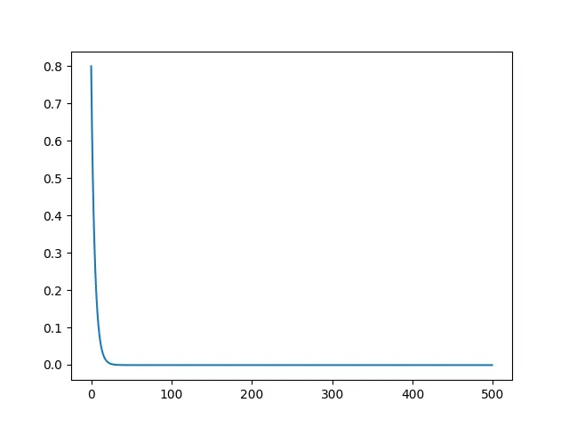
For n=500
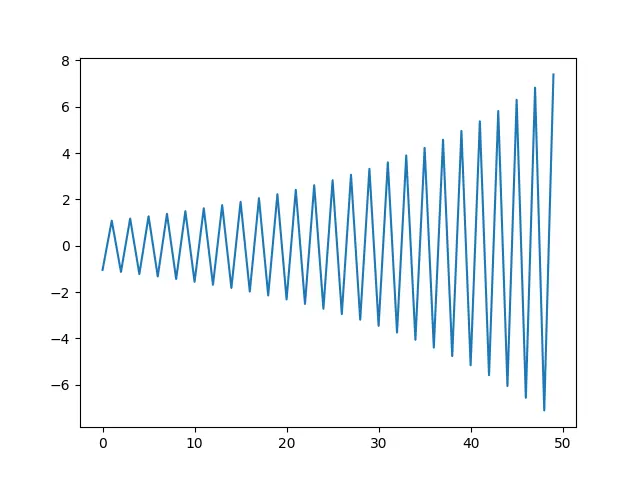
For n=50
Implicit form:
The python code is given below
"""
Implicit method

the differential equation is given as
dy/dx=-1000*y-exp(-x)
y(i+1)=y(i)-hexp(-x(i)+1)/[1+1000h]

"""
import matplotlib.pyplot as plt
import numpy as np
import math

x_0=0
x_end=0.1
n=50
h=(x_end-x_0)/(n-1)
x_initial=0
y_initial=1
y_final=[]

for i in range(0,n):

	x_initial=x_initial+h
	ans=(y_initial-(h*math.exp(-x_initial)))/(1+1000*h)
	y_initial=ans
	y_final.append(ans)

plt.plot(y_final)
plt.show()
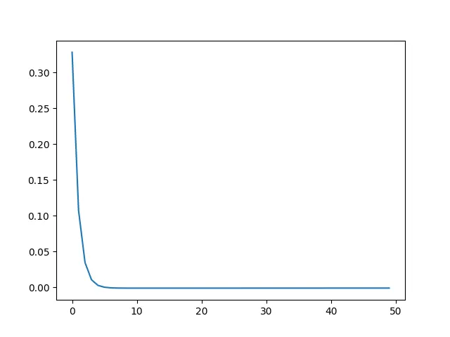
For n=50
Conclusion:
- In ODE becomes unstable in case of explicit scheme when the no of sub interval are lesser the scheme are unstable. Implicit schemes on the other hand is always stable.
- In engg simulation, there will be always an error associated with it, this error should be bounded throughout the simulation. So stability is important to consider for a cfd simulation.