Week 10: Project 1 - FULL HYDRO case set up (PFI)

Abstract:

This project deals with hydro case setup of PFI engine. In this both spray modelling and turbulent modelling are considered to analyse different characteristic parameters. Fixed embedding and adaptive mesh refinement techniques are used to refine the localised mesh at different regions which includes valves, combustion liners and nozzles. Emission characteristic plot of nox , soot, co2 and co emissions are predicted after combustion. Regions initialization are provided at different conditions. Overall, the performance specifications of PFI engines are analysed and further scope of developing the engine has been kept in view.

Aim:

To setup a complete hydro simulation of a PFI engine.

Introduction:

In Internal Combustion engine the intake manifold is the part of the engine between the Cylinders and the throttle body. In a multi-cylinder engine its primary purpose is to evenly distribute the air flow between each cylinder, and to create the homogeneous fuel air mixture. The mass flow rate of air which is entering in the engines cylinders plays a large impact on the volumetric efficiency. There are two types of fuel injection systems Single Point Fuel Injection (SPFI) and Multi Point Fuel Injection (MPFI) System. Multi-point, or multi-port is when there is a fuel injector for each cylinder and they are located as close as possible to the intake valve. These systems allow the engine management computer to hit a desired air fuel ratio very accurately for each cylinder. Multipoint fuel injection devotes a separate injector nozzle to each cylinder, right outside its intake port, which is why the system is sometimes called port injection. Shooting the fuel vapour this close to the intake port almost ensures that it will be drawn completely into the cylinder. The main advantage is that MPFI meters fuel more precisely than do TBI designs, better achieving the desired air-fuel ratio and improving all related aspects.

Function of injection system:

1. Accurate metering of the fuel injected per cycle: The quantity of the fuel metered should vary to meet changing speed and load requirements of the engine
2. Timing the injection of the fuel correctly in the cycle: to obtain maximum power ensuring fuel economy and clean burning

iii. Proper control of rate of injection: The desired heat release pattern is achieved during combustion

1. Proper atomization of fuel into very fine droplets.
2. Proper spray pattern to ensure rapid mixing of fuel and air
3. Uniform distribution of fuel droplets throughout the combustion chamber.

PFI is used when fuel (gasoline or diesel fuel) is injected before the valve and the cylinder when the combustion happens. The intake valve will have a fuel injection system that spray fuel into the air while coming into the combustion chamber. A spark plug is attached which ignites the mass of fuel and air in a right proportionate, pushing the piston down by expanding the cylinder and rotating the crankshaft.

DESIGN SPECIFICATION FOR SETTING UP PARAMETERS:

Engine Geometric Parameters

1. Bore =0.086 m
2. Stroke = 0.09 m
3. Connecting rod length = 0.18 m
4. RPM = 3000

Run parameters

1. Simulation mode: No Hydro

Simulation time parameters

1. Start time : -520 deg
2. end time : 120 deg

Boundary conditions

1. Piston temperature - 450K
2. Liner temperature - 450K
3. Head temperature - 450K
4. Spark Plug temperature - 550K
5. Spark Plug electrode temperature - 600K
6. Exhaust ports temperature - 500K
7. Exhaut outflow - 1 bar
8. Exhaust outlflow temperature - 800k
9. Exhaust species concentration - Calculate the stoichiometric condition
10. Exhaust valve top temperature - 525K
11. Exhaust valve angle temperature - 525K
12. Exhaust valve bottom temeprature - 525K
13. Intake port - 1 temperature 425K
14. Intake port - 2 temperature 425K
15. Inflow pressure - 1 bar total pressure
16. Inflow temperature - 363K
17. Inflow species - Air
18. Intake valve top temperature - 480K
19. Intake valve angle temperature - 480K
20. Intake valve bottom temeprature - 480K

Initial conditions

• Intake port - 1 (closer to combustion chamber)
  • ic8h18 - 0.025508
  • o2 - 0.20157
  • n2 - 0.77292
  • Temperature - 390k
  • pressure - 1 bar
• Intake port - 2 (away from combustion chamber)
  • Air
  • Temperature - 370K
  • Pressure - 1 bar
• Cylinder
  • Pressure - 1.85731 bar
  • Temperature - 1360K
  • Stoichiometric composition

Injection Parameters

1. Fuel flow rate = 7.5e-4 Kg/second
2. Injection start time = -480.0
3. Injection duration = 191.2
4. Fuel temperature = 330K

Nozzle positions

Nozzle diameter = 250 micro-meter

Circular injection radius = Nozzle radius

Spray cone angle = 10

• Nozzle 0
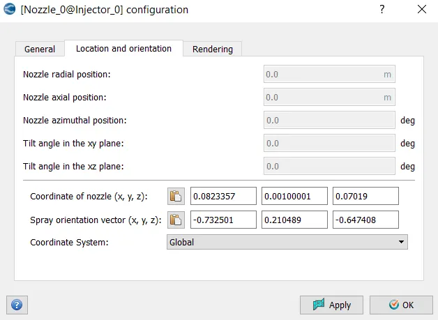
  • center 0.0823357 0.00100001 0.07019
  • Align Vector -0.732501 0.210489 -0.647408
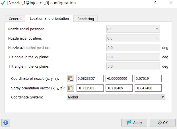
• Nozzle 1
  • center 0.0823357 -0.00099999 0.07019
  • Align Vector -0.732501 -0.210489 -0.647408
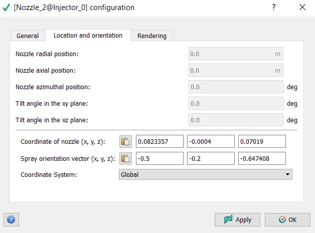
• Nozzle 2
  • center 0.0823357 -0.0004 0.07019
  • Align Vector -0.5 -0.2 -0.647408
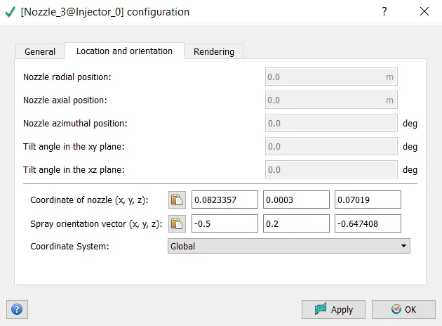
• Nozzle 3
  • center 0.0823357 0.0003 0.07019
  • Align Vector -0.5 0.2 -0.647408

Spark Ignition Parameters

• Start of spark = -15 deg
• Spark duration = 10 deg
• Spark location = -0.003 0 0.0091
• Spark radius = 0.0005m

OBJECTIVE:

1. What is the compression ratio of this engine?

2. Why do we need a wall heat transfer model? Why can't we predict the wall temperature from the CFD simulation?

3. Calculate the combustion efficiency of this engine

4. use the engine performance calculator, to determine the power and torque for this engine.

NOTE : Since Work and Torque has the same unit (N-m) , it doesn't mean value for Torque and Work will be the same.

Both are different quantities and has totally different meaning.

So the value for work that you will be getting from the engine performance calculator is not the value for the torque.

Calculate the value for the torque using the formula as shown below,

Power(P) = (2*π*N*T)/60

5. What is the significance of ca10, ca50 and ca90?

Table for boundaries assigned with different regions

Boundary flag	Region names
Piston	Cylinder region
Cylinder head	Cylinder region
Liner	Cylinder region
Spark plug	Cylinder region
Spark plug terminal	Cylinder region
Outflow	Exhaust region
Exhaust port	Exhaust region
Exhaust valve top	Exhaust region
Exhaust valve angle	Exhaust region
Exhaust valve bottom	Cylinder region
Inflow	Intake port 2
Inlet port 1	Intake port 1
Inlet port 2	Intake port 2
Intake valve top	Intake port 1
Intake valve angle	Intake port 1
Intake valve bottom	Cylinder region

Geometrical preparation and boundary flagging:

Open the converge studio panel

Import the model stl file format and on clicking the diagnosis tab errors are seen

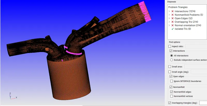
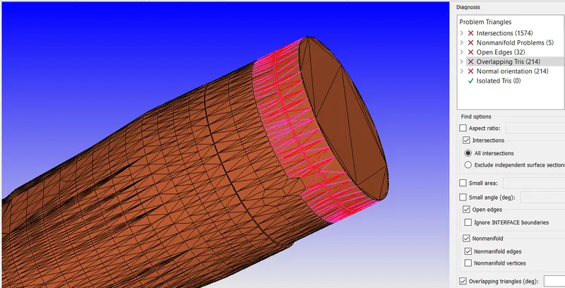
Intersection error:

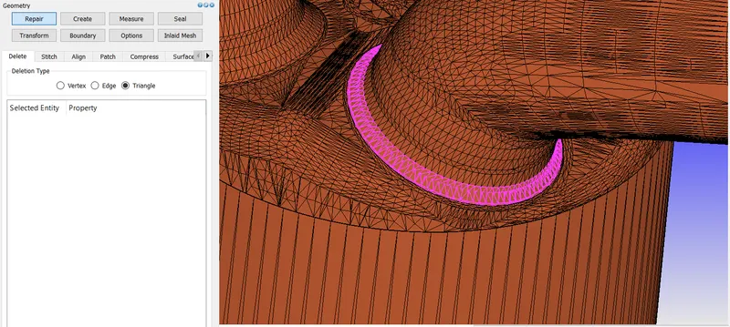
Inlet valve is so high that it is passing through cylinder head. To fix the problem, we need to push back the valve in the right location.

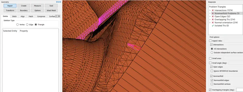
Non manifold problem

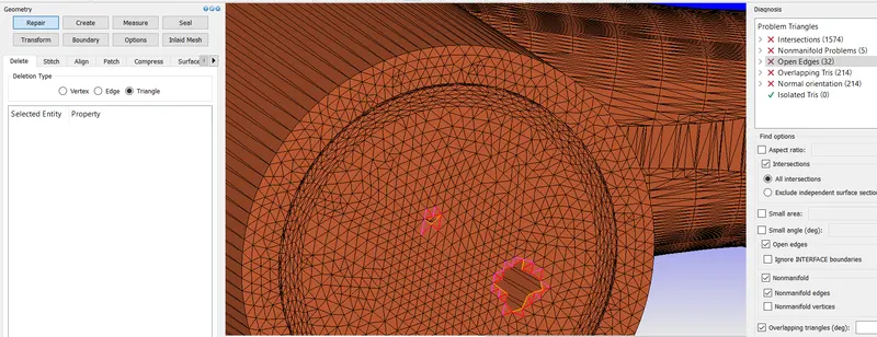
Open edge problem

Overlapping error

Boundary flagging:

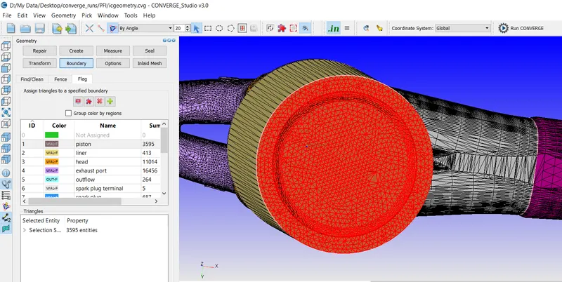
piston

select triangle entity with any angle selection>> Select the bootom portion of geometry> Assign to piston boundary and apply

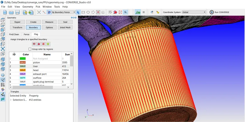
liner

boundary>fence> select edge by arc option> select 2 arc on the top and bottom of the cylinder.

after creating fence, select triangle entity selection with boundary fence> select triangles behind the fences and assign them to liner boundary

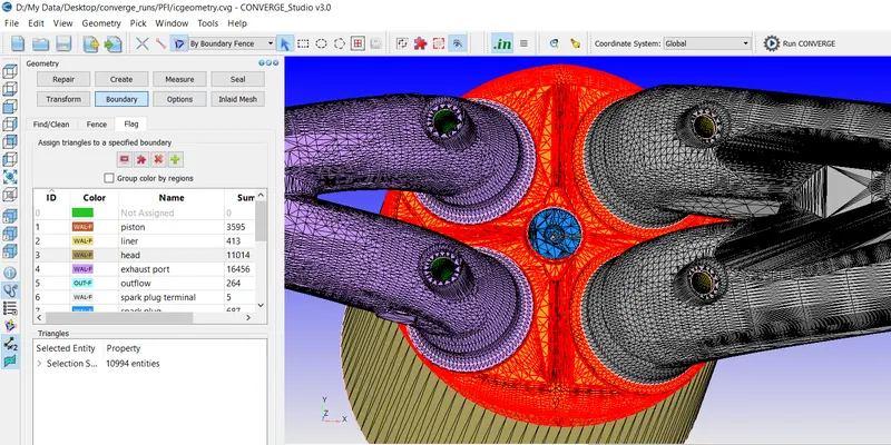
Cylinder head

create boundary fence to assign triangles at the desired boundary

Boundary> fence> By selected edge with arc option, select 5 arc i.e 4 arc on the port and one at the cylinder

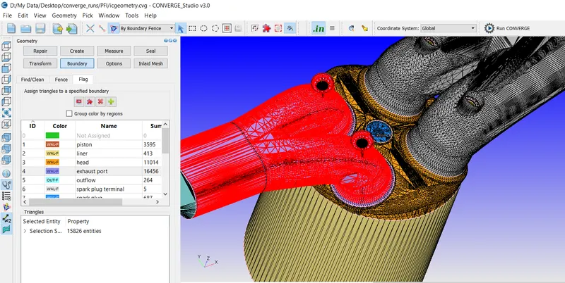
Exhaust port

choose triangle entity with any angle with 20 degree>>select the triangles on the exhaust port and assign them

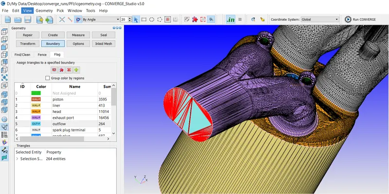
Outflow

choose triangle entity with any angle with 20 degree>>select the triangles on the outer face of exhaust portand assign them

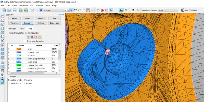
Spark plug terminal

select triangle entity with boundary fence selection> select the triangles inside the small fence> assign them to spark plug terminal and then apply.

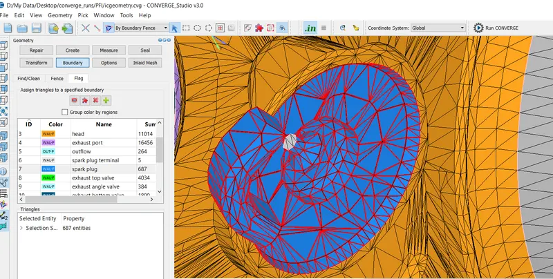
Spark plug

boundary> fence> select edge by arc option> select two arc i.e one for spark plug and other for spark terminal> mark fence

After creating fence select triangle entity as boundary fence > select the triangles on the inner side of the cylinder head except the triangle inside the small fence.

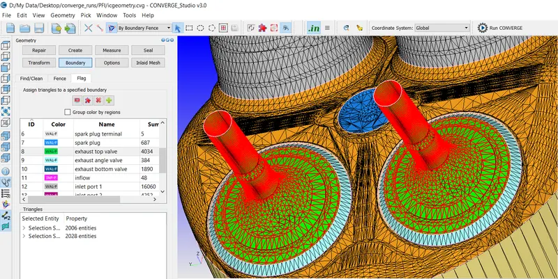
Exhaust valve top

first of all we divide the valve in three parts to assign different boundaries

boundary> fence> select edge by arc option>select 3 edges and mark the fence

after mark fence, select triangle entity by boundary fence method> select triangle between the top and the middle fence>> assign them exhaust top boundary

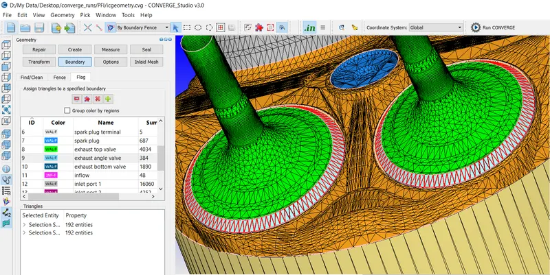
Exhaust valve angle

choose triangle entity with any angle with 20 degree>>select the triangles between the middle and the bottom create fence

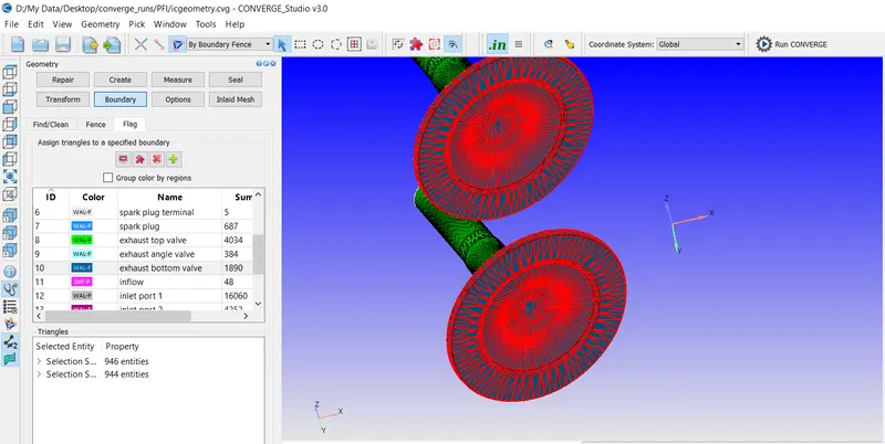
Exhaust valve bottom

choose triangle entity with any angle with 20 degree>>select the triangles at the bottom face of the valve

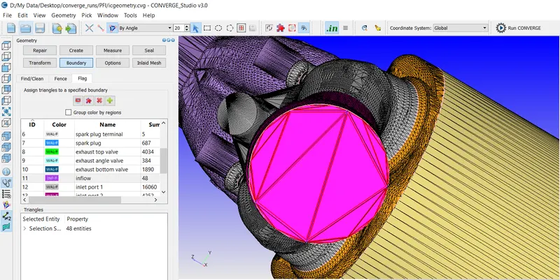
Inflow

choose triangle entity selection by angle method 20> select triangle on the exit face and assign them

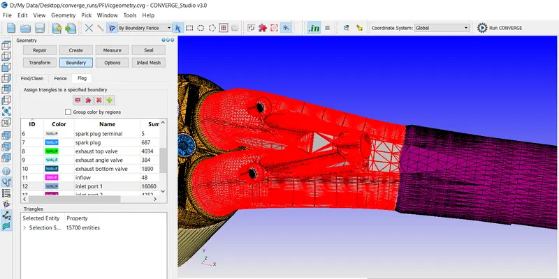
Inlet port 1

boundary> fence> reconstructing fence from existing boundaries

this will create fence from the existing boundaries

choose triangle entity by selecting the boundary fence option> select the triangles and assign them

Inlet port 2

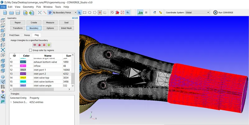
boundary> fence> reconstruct fence from existing boundaries. This marks fence from boundary region.

boundary> fence> select edge by arc option and select the triangles over the regions

Inlet valve top

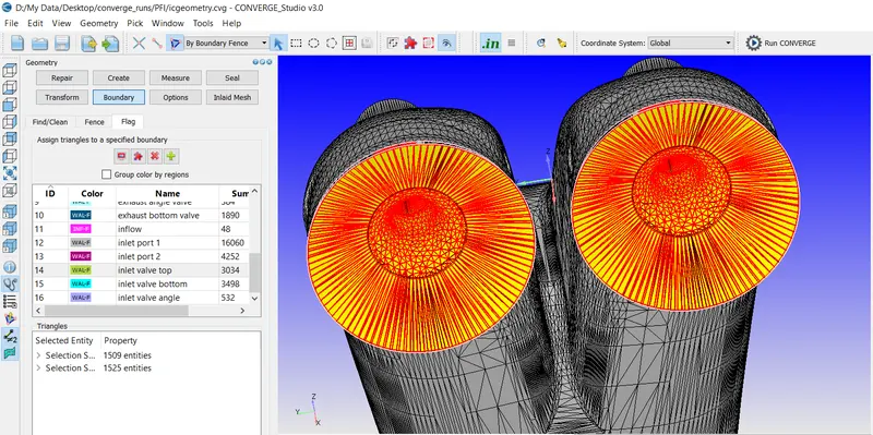
boundary> fence> reconstruct fence from existing boundaries. This marks fence from boundary region and also seperate the ring triangles from the valve.

select triangle entity as boundary fence>> select the triangles and then assign them

Inlet valve bottom

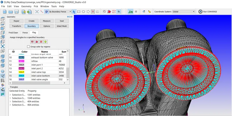
choose triangle entity with any angle with 20 degree>>select the triangles on the bottom of the intake valve region

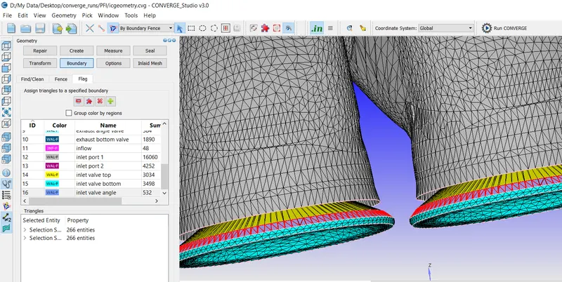
Intake valve angle

boundary> fence> reconstruct fence from existing boundaries. This marks fence from boundary region.

boundary> fence> select edge by arc option and select two arc to assign them

Valves:

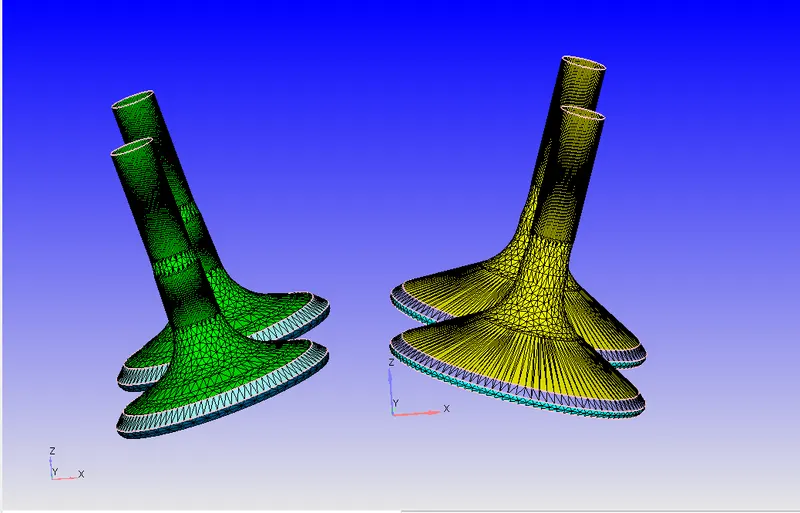
Ring triangles

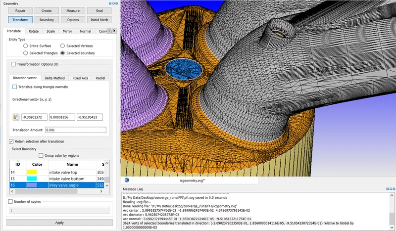
Ring triangles are selected and are provided to make the valve move smoothly without distorting the geometry of the port.

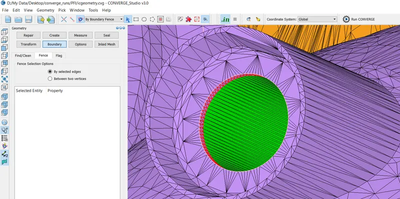
boundary> select fence> create fence on the top region> select triangle entity with boundary fence option and apply to the respective port

To remove the open edge errors

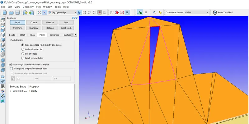
delete the overlapping triangles>> select the openedges> got to patch> auto assign boundaries for triangles

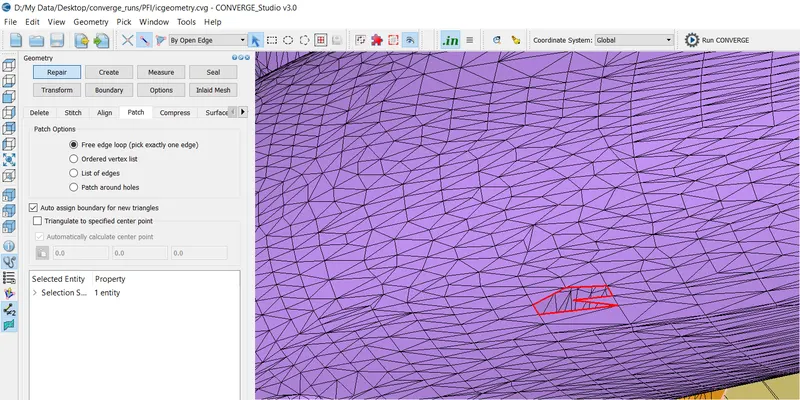
Normal orientation

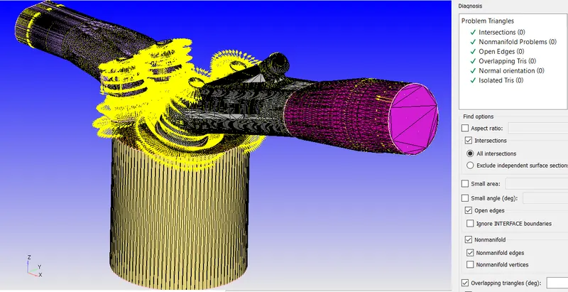
final clean geometry

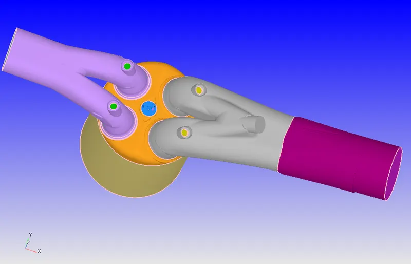
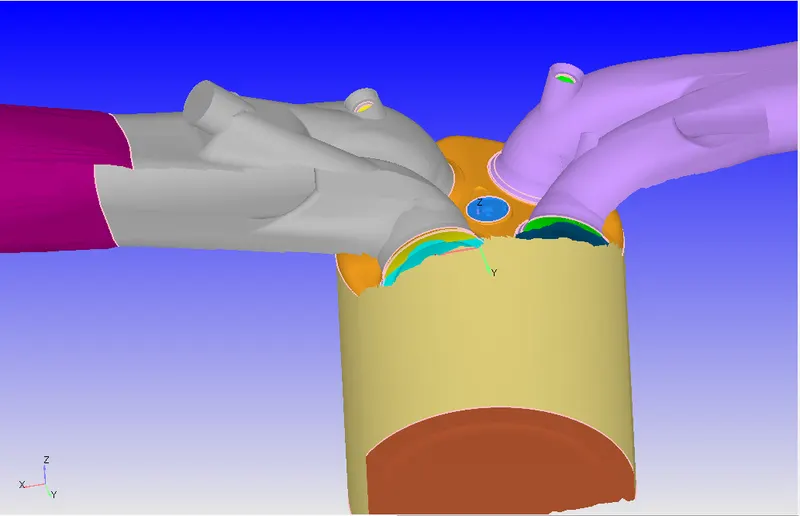
Cut view of PFI engine

Simulation case setup:

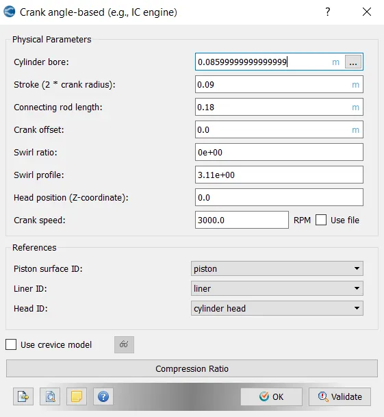
Application:

Type- crank angle based IC engine

Details of IC engine

Cylinder bore: 0.0856m

Stroke length: 0.09m

Connecting rod: 0.18m

Crank speed: 3000rpm

Piston surface ID: piston

Liner ID: LINER

Head ID: cylinder head

Parcel simulation:

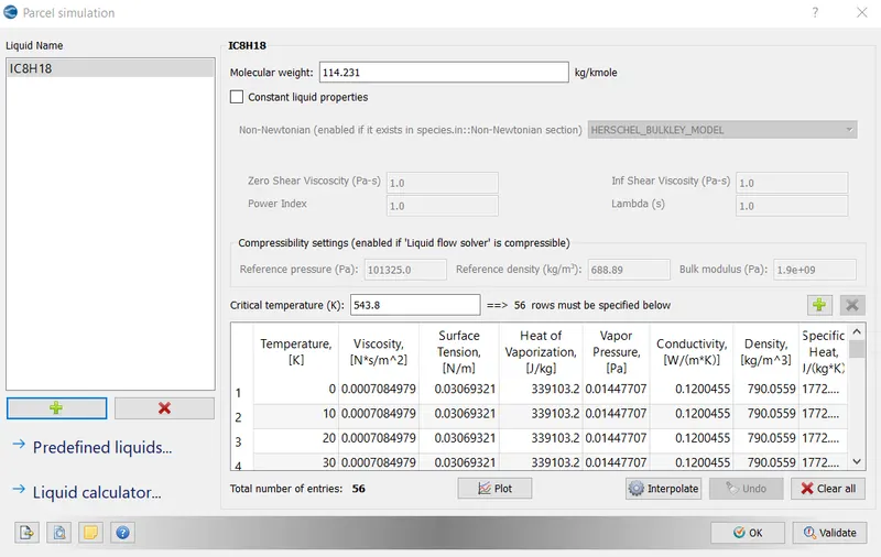
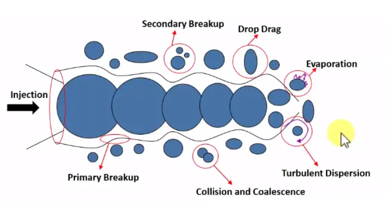
Parcel refers to Lagrangian based spray model. Parcel undergoes several physical process like primary breakup, secondary breakup, drop drag, coalescence and collision, evaporation etc. parcel statistically determines the fuel spray.

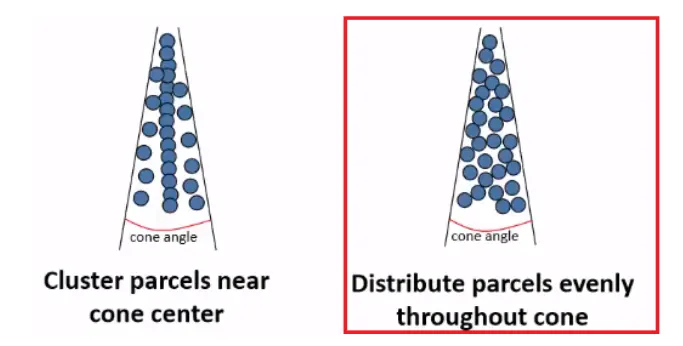
Parcel distribution can be identified in two ways:

• Cluster parcel near cone
• Distribute parcels evenly throughout cone

Isooctane IC8H18 is chosen as a parcel, which will act as a fuel medium for combustion.

Select Add option> choose isooctane> check validate and the ok

Materials:

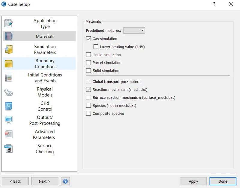
Enable reaction mechanism option

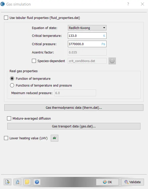
Gas simulation:

Select the gas thermodynamic data>> select import data from therm.dat>>load the therm.dat file

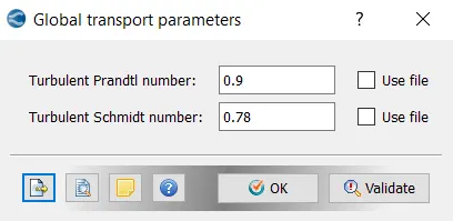
Global transport parameters:

Select default settings

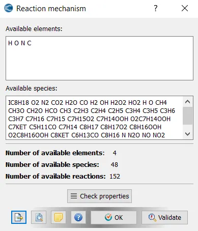
Reaction mechanism:

Select data from mech.dat file>> load the mech.dat file containing all the reacting species

Click on check properties. The following message will pop up ‘no errors found’

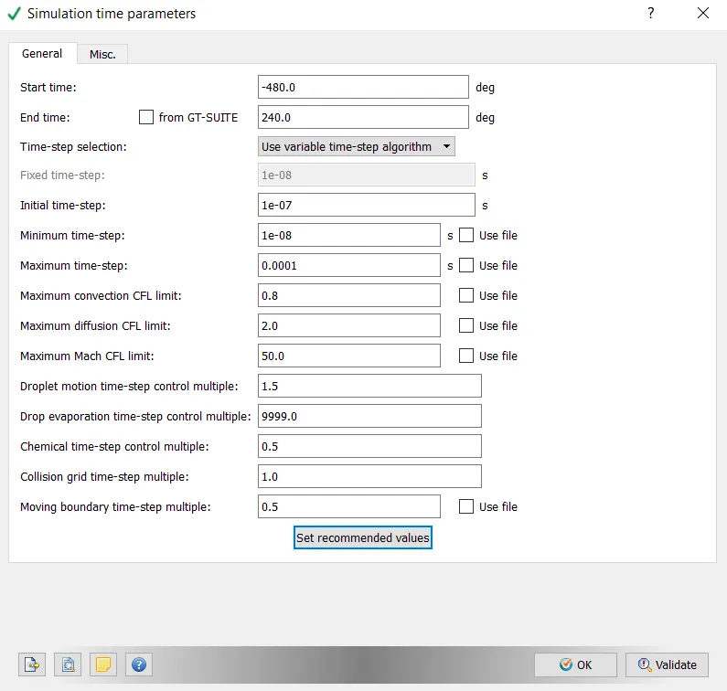
Simulation parameters:

Run parameters:

Solver- transient

Temporal type- crank angle based engine simulation

Simulation time parameter:

Start crank angle: -480 degree

End crank angle: 240 degree

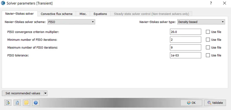
Solver parameter:

Navier-Stokes solver type: density based

Boundary conditions:

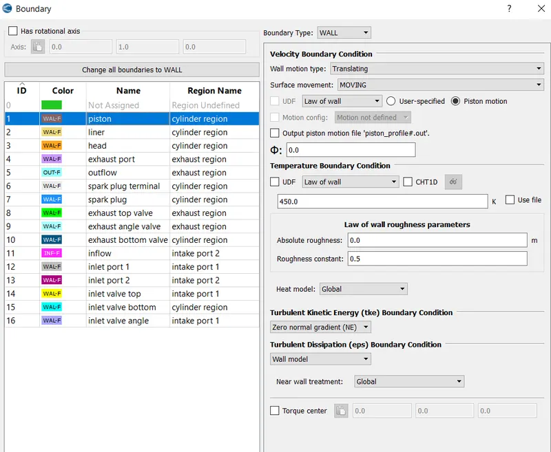
Piston:

Boundary type- wall

Wall motion- translating, law of wall, piston motion

Temperature: 450k, law of wall

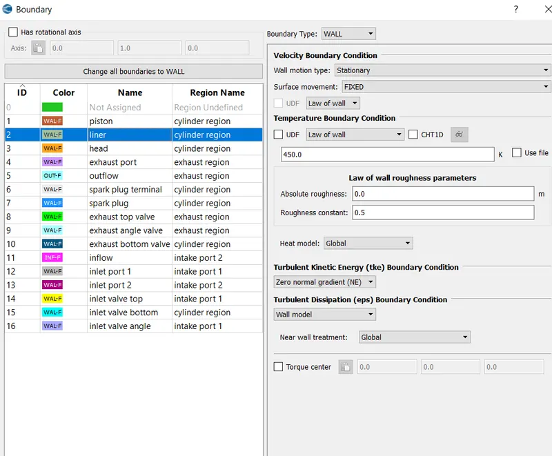
Liner:

Boundary type: wall

Wall motion: stationary, fixed, law of wall

Temperature: 450k, law of wall

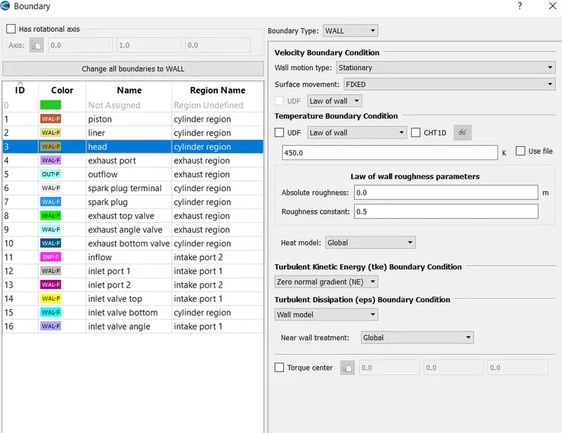
Cylinder head:

Boundary type: wall

Wall motion: stationary, fixed, law of wall

Temperature: 450k, law of wall

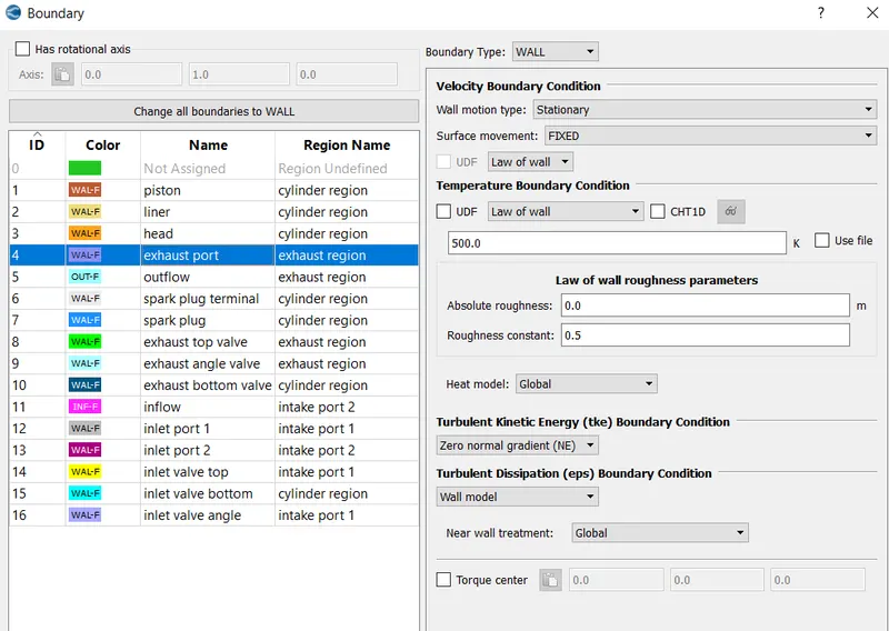
Exhaust port:

Boundary type: wall

Wall motion: stationary, fixed, law of wall

Temperature: 500k, law of wall

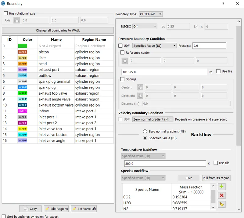
Outflow:

Boundary type: outflow

Pressure: 101325Pa

Temperature backflow: 800k

Species backflow: Stoichiometric species

Stoichiometric calculation:

Species	Mass fraction
CO2	0.192304
H2O	0.088559
N2	0.719137

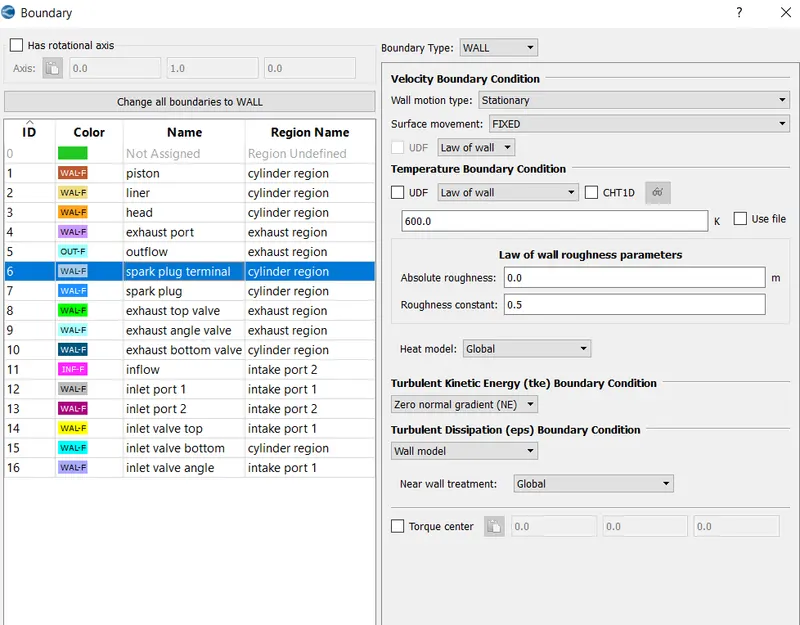
Spark plug terminal:

Boundary type: wall

Wall motion: stationary, fixed, law of wall

Temperature: 600k, law of wall

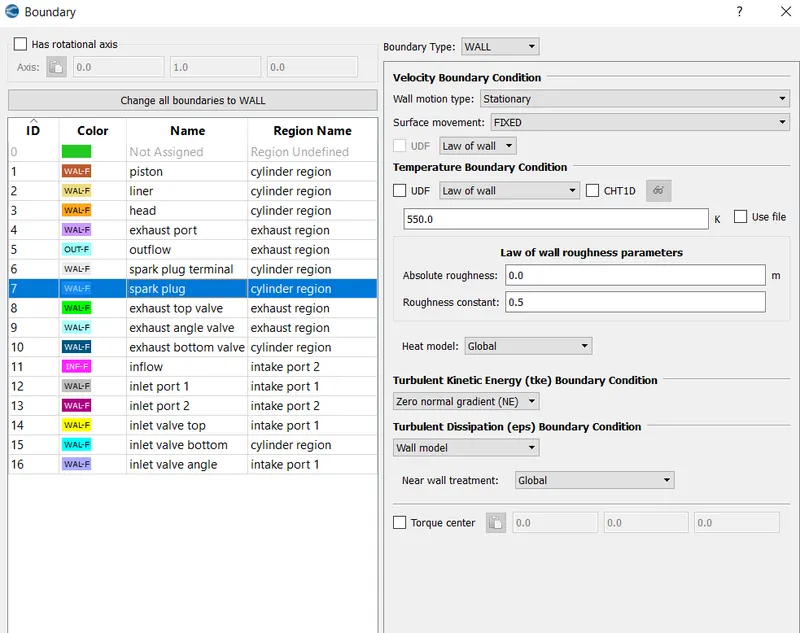
Spark plug:

Boundary type: wall

Wall motion: stationary, fixed, law of wall

Temperature: 550k, law of wall

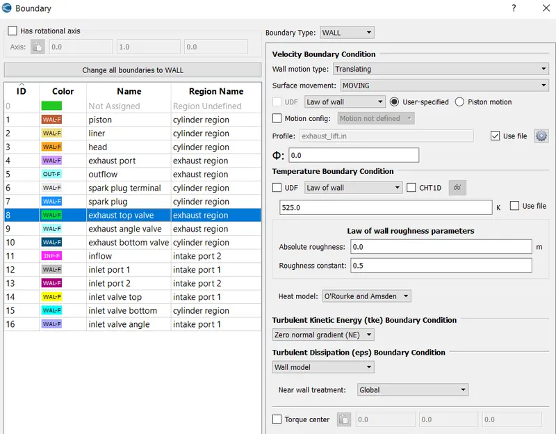
Exhaust valve top:

Boundary type: wall

Wall motion: translating

Surface movement: moving

Temperature: 525k, law of wall

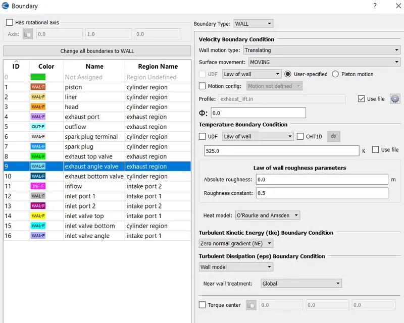
Exhaust valve angle:

Boundary type: wall

Wall motion: translating

Surface movement: moving

Temperature: 525k, law of wall

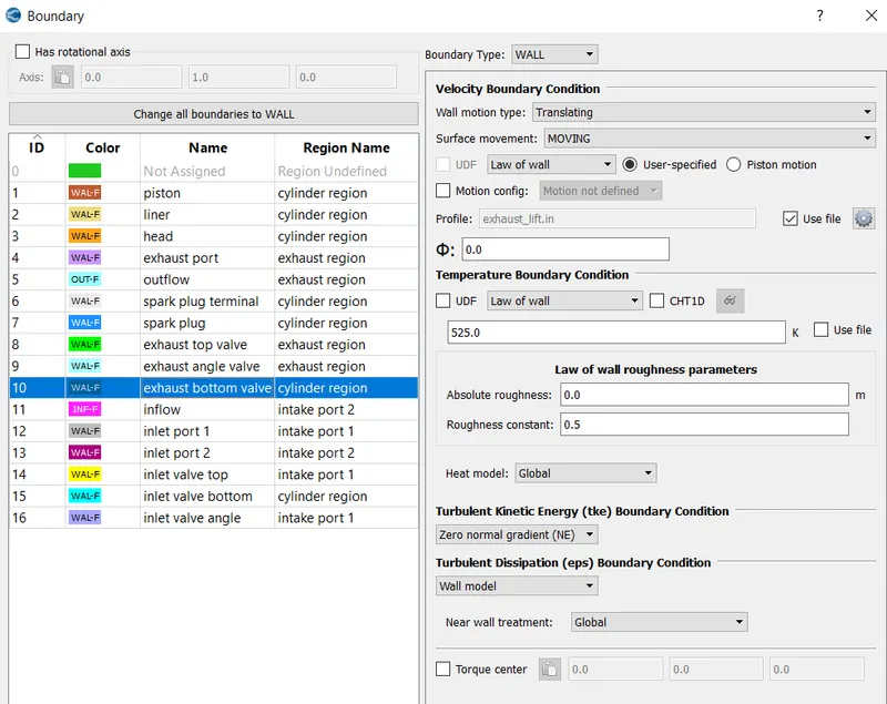
Exhaust valve bottom:

Boundary type: wall

Wall motion: translating

Surface movement: moving

Temperature: 525k, law of wall

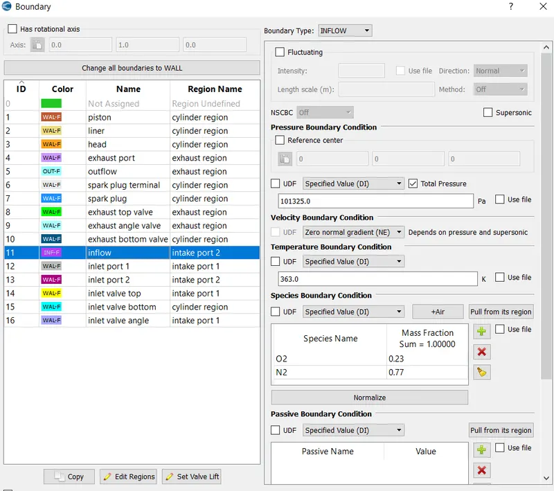
Inflow:

Boundary type: inflow

Pressure: 101325Pa

Temperature: 363k

Species: air

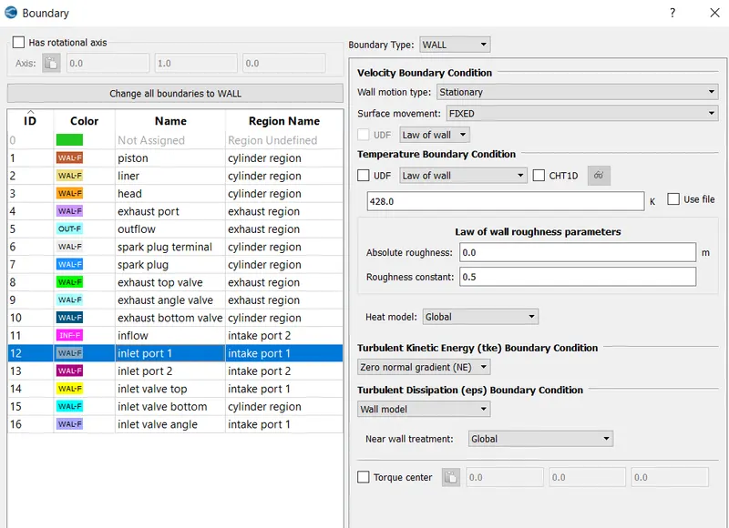
Inlet port 1:

Boundary type: wall

Wall motion: stationary, fixed, law of wall

Temperature: 428k, law of wall

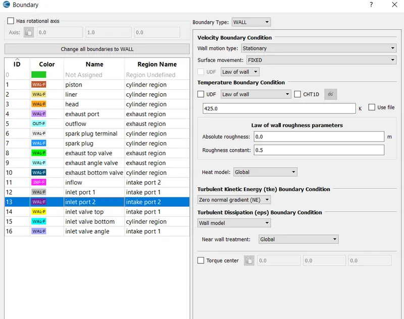
Inlet port 2:

Boundary type: wall

Wall motion: stationary, fixed, law of wall

Temperature: 425k, law of wall

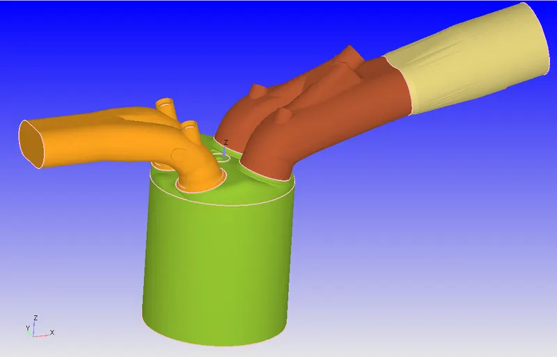
The inlet port is split in two boundaries and also in two separate regions to provide different boundary conditions. The intake port 1 is where the fuel spray is injected.

When the intake valve is closed, some amount of spray are present on one half of the intake port, whereas in other half there are no spray parcel. To initialize some amount of fuel in the intake port that is closer to the combustion chamber, we need to split the intake port into 2 boundaries.

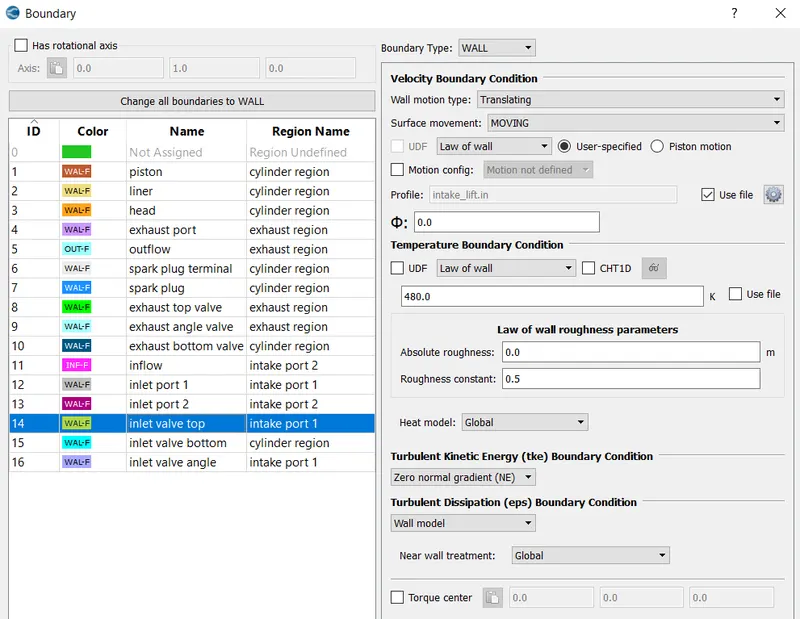
Intake valve top:

Boundary type: wall

Wall motion: translating

Surface movement: moving

Temperature: 480k, law of wall

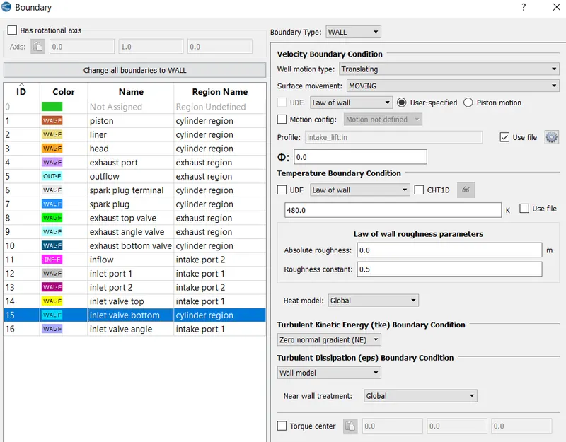
Intake valve bottom:

Boundary type: wall

Wall motion: translating

Surface movement: moving

Temperature: 480k, law of wall

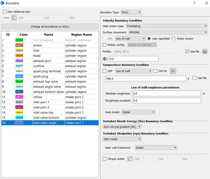
Inlet valve angle:

Boundary type: wall

Wall motion: translating

Surface movement: moving

Temperature: 480k, law of wall

Initial conditions and events:

Enable the event option

Select regions and initialization

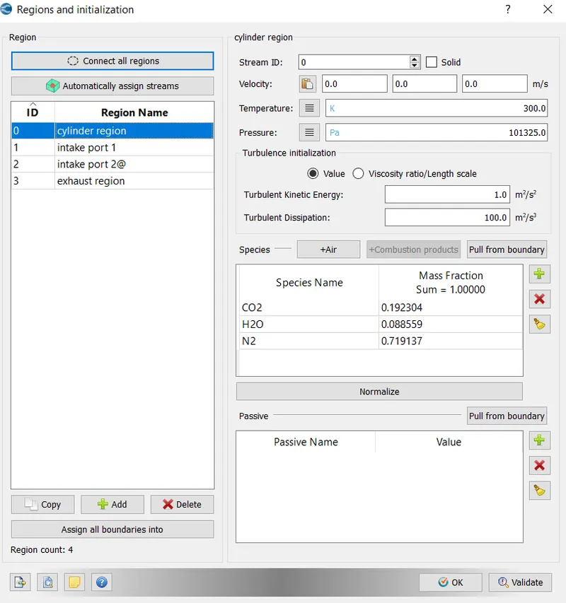
Region 0: cylinder region

Temperature-300k

Pressure-101325Pa

Species	Mass fraction
CO2	0.192304
H2O	0.088559
N2	0.719137

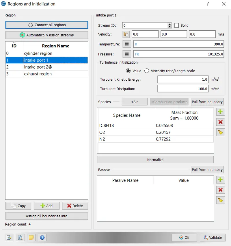
Region 1: Intake port 1

Temperature-300k

Pressure-101325Pa

Species	Mass fraction
CO2	0.192304
H2O	0.088559
N2	0.719137

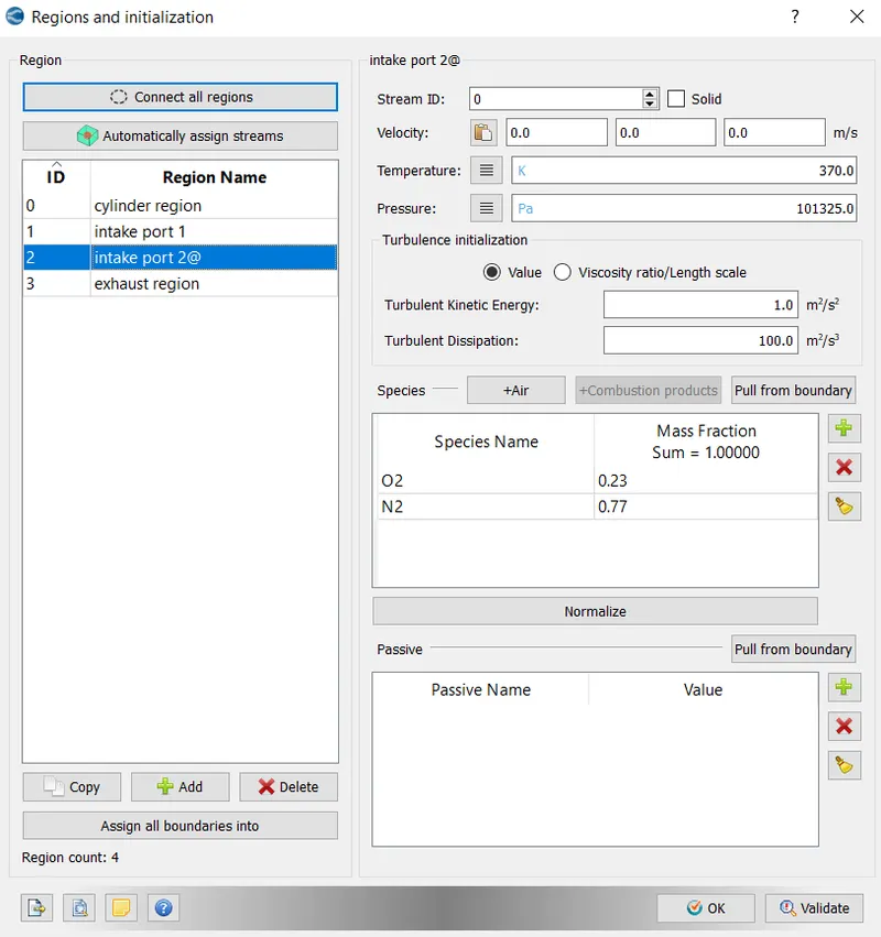
Region 2: Intake port 2

Temperature-370k

Pressure-101325Pa

Species: air

Region 0: Exhaust region

Temperature-1360k

Pressure-185731Pa

Species	Mass fraction
CO2	0.192304
H2O	0.088559
N2	0.719137

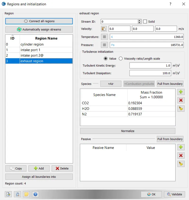
Region based PFI engine:

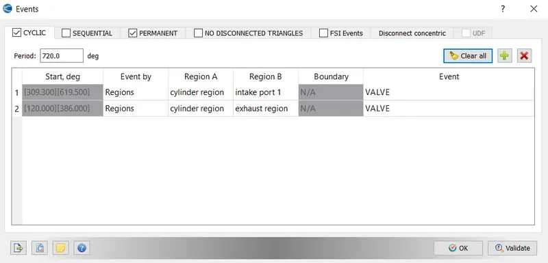
Events:

Cyclic events

First event:

Region A- cylinder region

Region B- intake port 1

Event- valve

Second event:

Region A- cylinder region

Region B- exhaust region

Event- valve

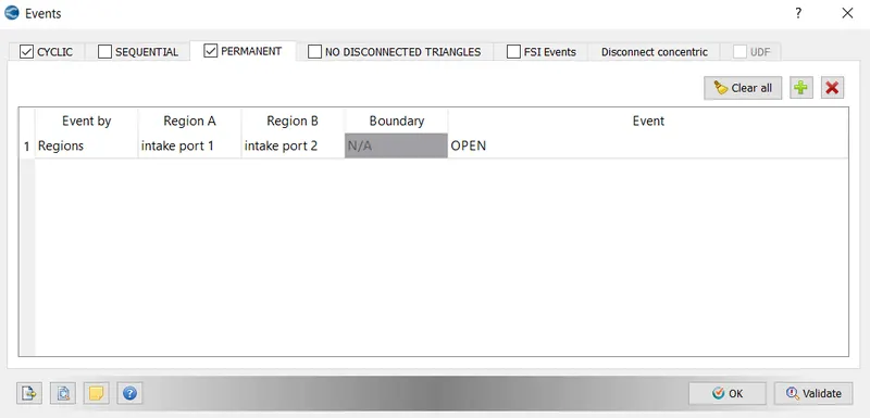
Permanent event

Region A- intake port 1

Region B- intake port 2

Event- open

Physical model

Spray modelling:

Spray modelling includes liquid atomization, drop breakup, collision, turbulent dispersion etc. in converge spray model of liquid droplet is done by lagrangian parcel method. In each drop of parcel, the mass, momentum, energy and heat transfer are solved. It is sometimes called discrete phase model or lagrangian model.

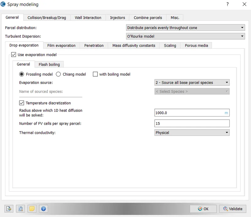
The general settings for the spray model is given below:

Parcel distribution: distribute parcel evenly throughout the cone

Turbulent dispersion: O’Rourke model

Drop evaporation> use evaporation model

Evaporation source: source all base parcel species

Enable temperature discretization

Radius above which ODE needs to be solved: 1000

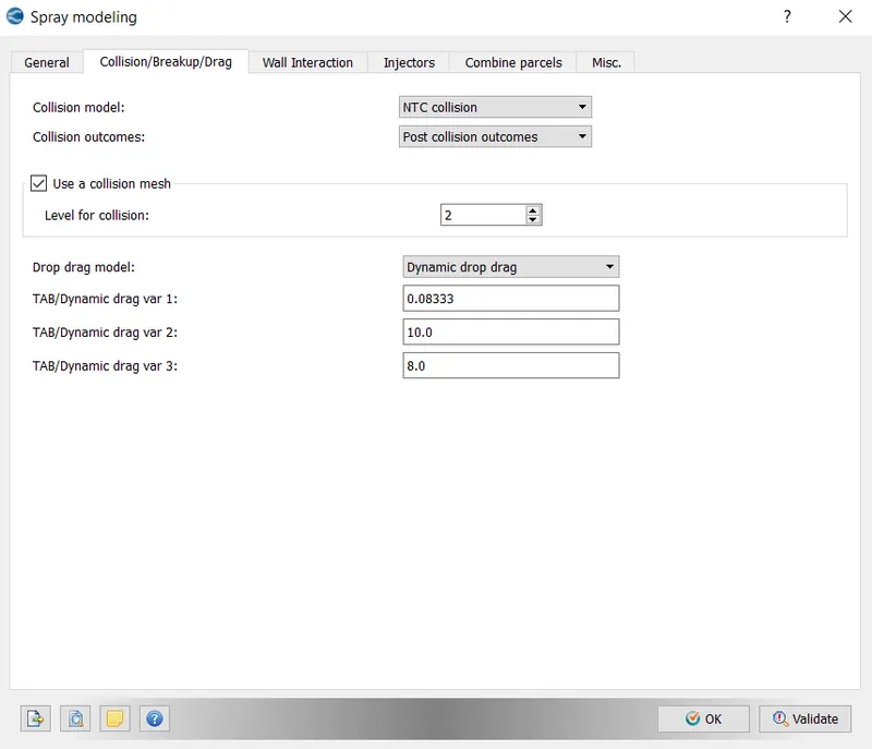
Collision model:

Model: NTC Model

Use collision mesh

Drop and drag model > select dynamic drop and drag model

Injectors:

Now we define the inputs to the injector parts.

Go to injectors> select the edit tab

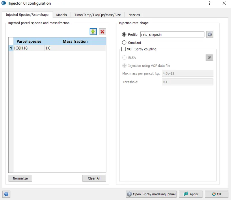
Injected species/ Rate shape

Select the parcel species as isooctane

Mass fraction: 1

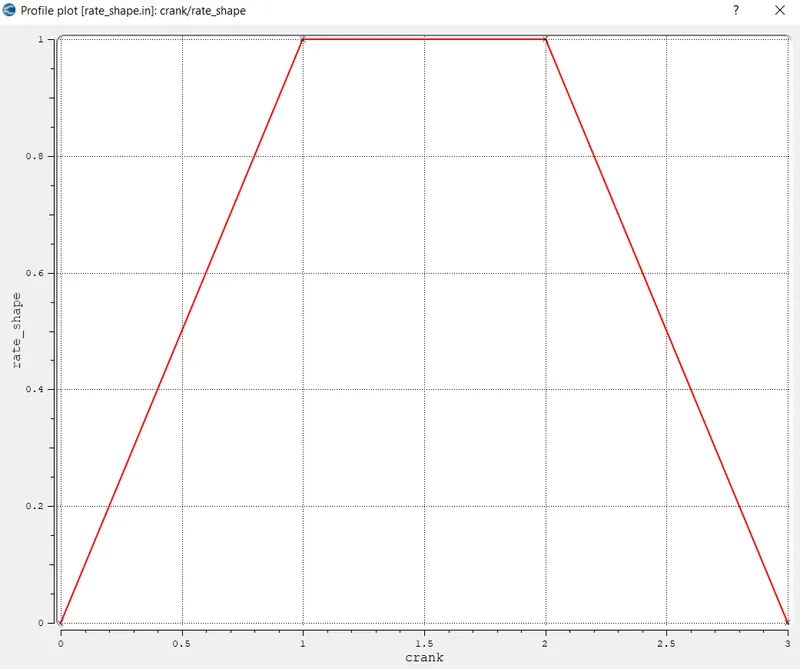
Injection rate shape:

We use the profile option to define the rate shape function with respect to the crank angle.

Save the file name as rate_shape.in format.

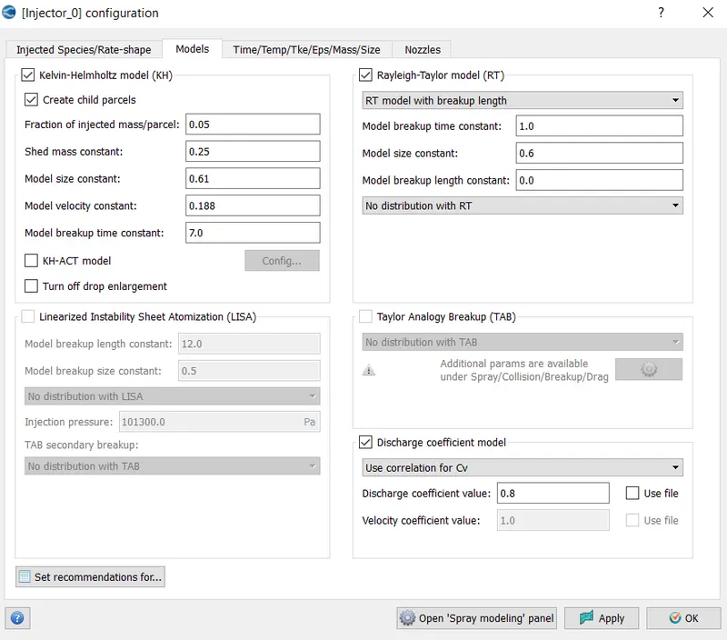
Models:

Activate the kelvin-Helmholtz model and Rayleigh-Taylor model.

Click on recommendation and choose gasoline PFI. Keep rest of the parameters as constant.

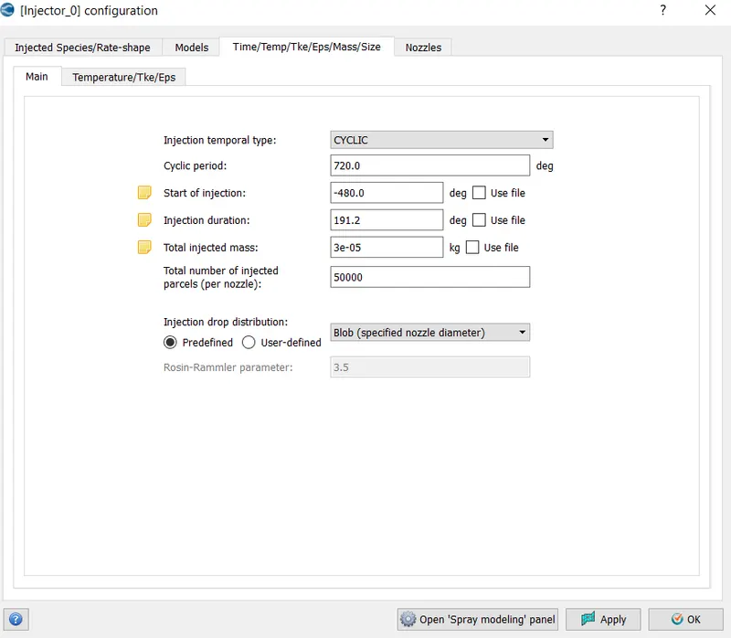
Time/temp/TKE/EPS/Mass/Size:

Go to the Main tab.

Injection temporal type: cyclic

Cyclic period: 720 degree

Start injection: -480 degree

Injection duration: 191.2 degree

Total injected mass: 3e-5

Computation of total injected mass

`RPM=3000`

`RPS=3000/60=50`

`DPS=RPS*360=50*360=18000`

`TIME PER DEGREE=1/DPS=1/18000=5.55e-5`

`TIME PER 720 DEGREE=(5.55e-5)*720=0.04`

`Total flow rate=7.5e-4`

`FUEL MASS PER CYCLE=Total flow rate*time per 720 degree=(7.5e-4)*0.04=3e-5 kg`

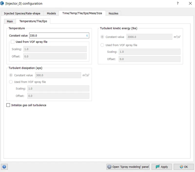
Temperature tab:

Temperature constant value: 330k

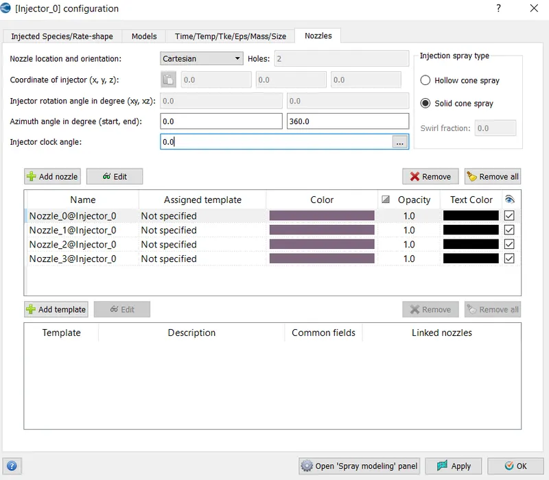
Nozzles:

We define the settings as given below.

Nozzle location and orientation: Cartesian

Click on the add nozzle tab and select the edit option.

General tab

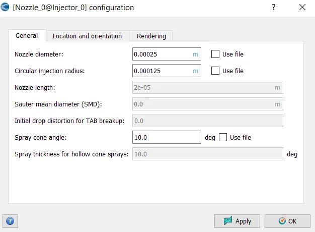
Injection nozzle 0

Nozzle diameter: 250e-6 m

Circular injection radius: 125e-6 m

Spray cone angle: 10 degree

Provide the location coordinate of nozzle.

Provide the spray orientation axis of the nozzle.

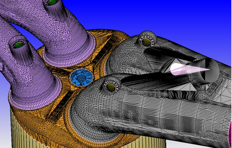
Injection nozzle 1

Nozzle diameter: 250e-6 m

Circular injection radius: 125e-6 m

Spray cone angle: 10 degree

Provide the location coordinate of nozzle.

Provide the spray orientation axis of the nozzle.

Injection nozzle 2

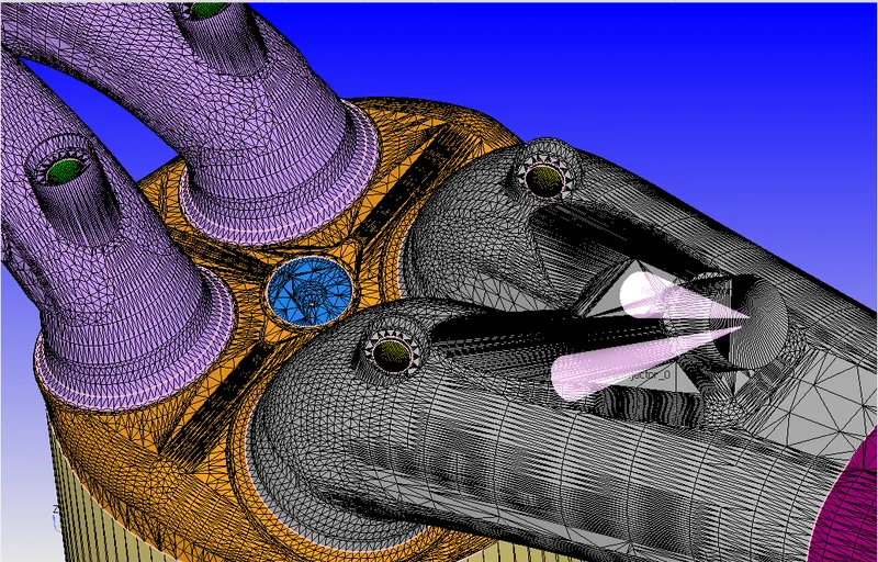
Nozzle diameter: 250e-6 m

Circular injection radius: 125e-6 m

Spray cone angle: 10 degree

Provide the location coordinate of nozzle.

Provide the spray orientation axis of the nozzle.

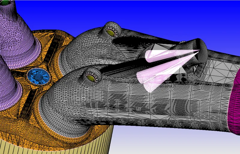
Injection nozzle 3

Nozzle diameter: 250e-6 m

Circular injection radius: 125e-6 m

Spray cone angle: 10 degree

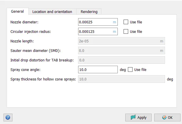
Provide the location coordinate of nozzle.

Provide the spray orientation axis of the nozzle.

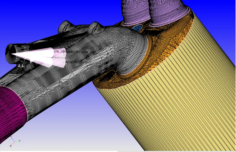
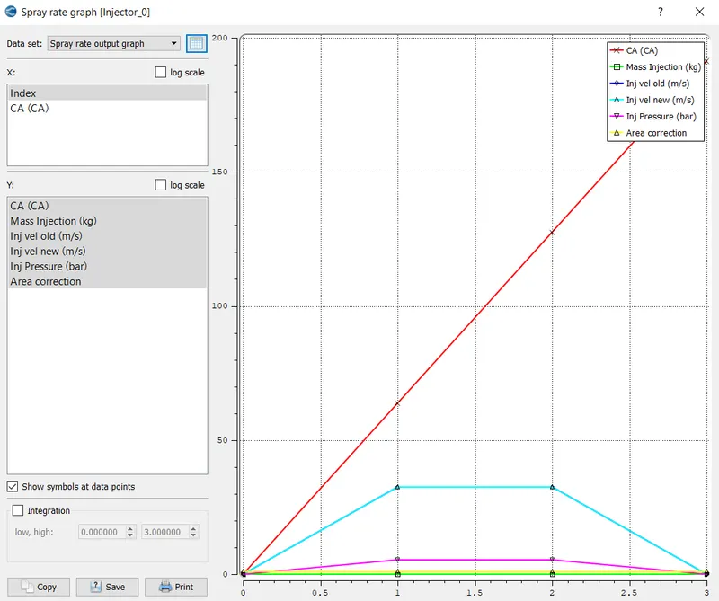
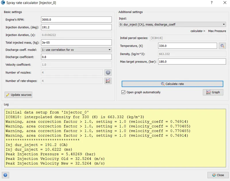
Now from the spray modelling tab, we check for preview of the spray rate and validate nozzle location.

Select tools> select spray rate preview> check all the settings and click on calculate rate.

The spray rate output graph is shown below

The output values are predicted below

Now go to tools option> select validate nozzle location. The following clear messages will appear on the screen.

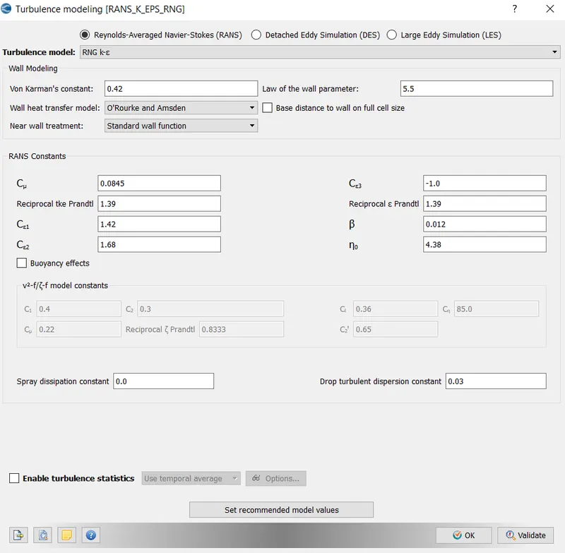
Turbulent model:

Choose RNG K-epsilon as turbulent model

Combustion modelling:

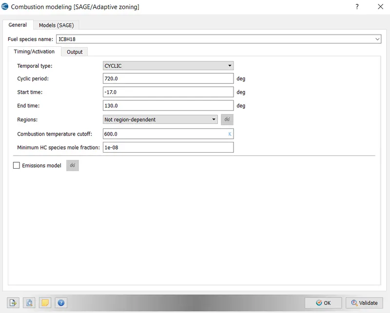
The combustion is modelled by the reaction mechanism. There are multiple intermediate species that govern the combustion reaction. The reaction mechanism is too large to simulate, so it is solved for those species whose presence are affected by combustion.

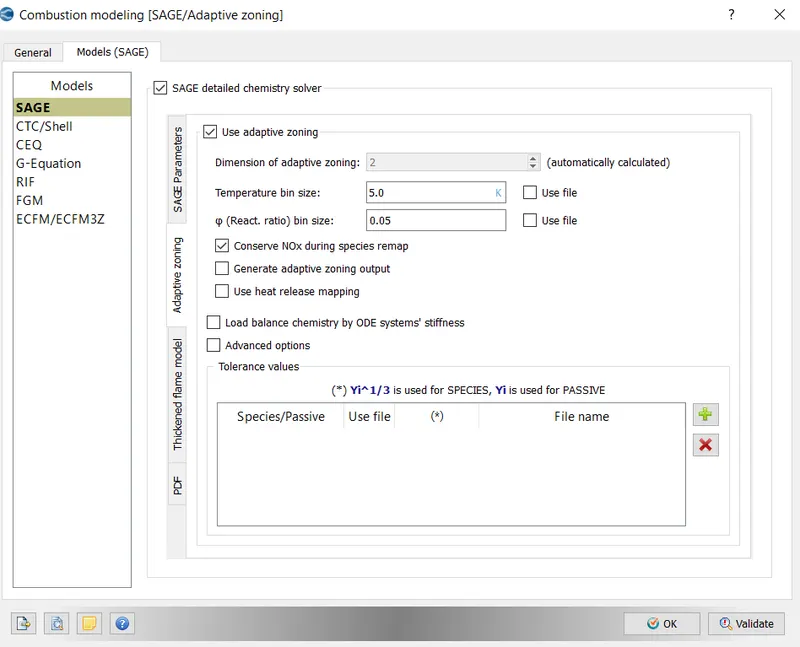
In combustion modelling SAGE chemistry solver is used. Some of the details regarding the solver is given below:

For General tab

Fuel species: IC8H18

Temporal type: cyclic

Cyclic period: 720 degree

Start:-17 degree

End: 130 degree

Combustion cut off temperature: 600k

Minimum HC species mole fraction: 1

Model tab

Models: SAGE modelling

Adaptive zoning: This technique helps converge to quickly simulate the flow field by speeding up species transport equation and reach an accurate limited phenomenon and emission.

Source/sink modelling:

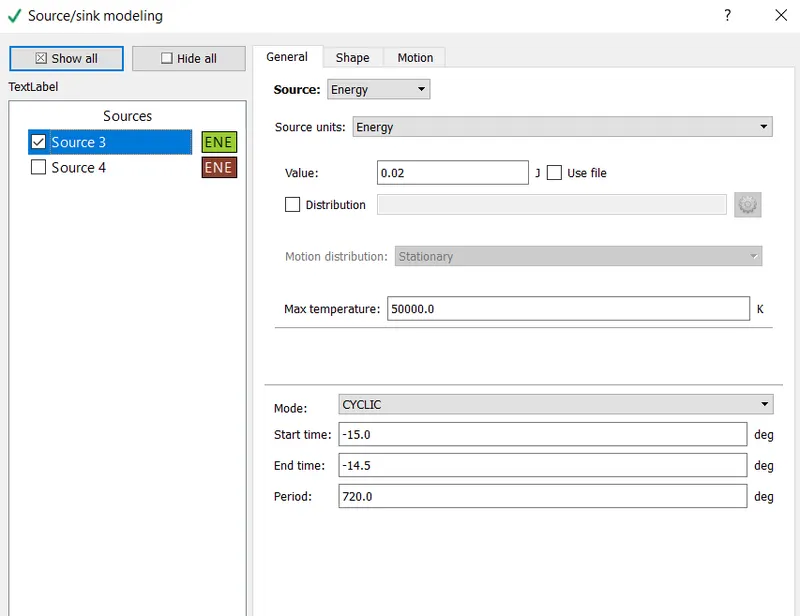
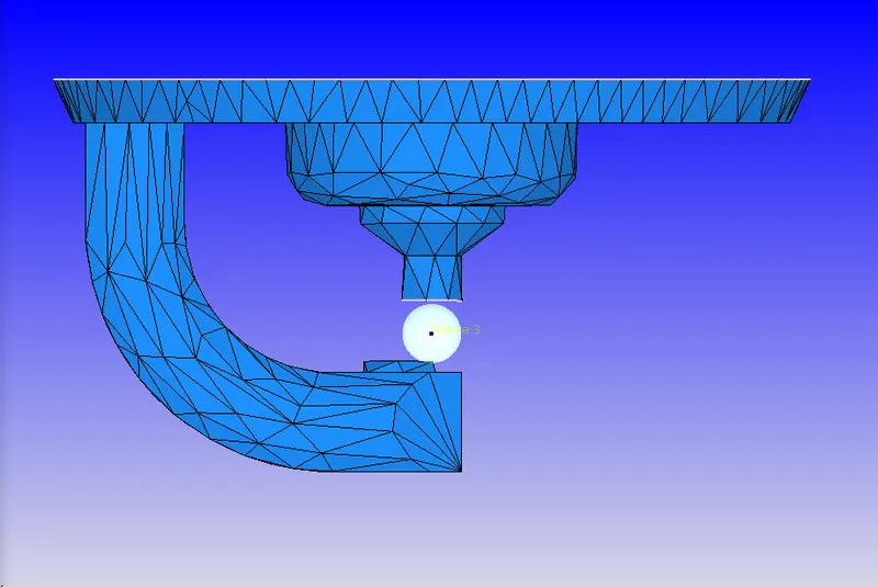
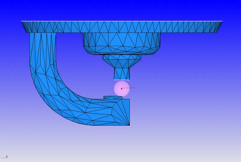
The spark plug and the spark plug terminal are at very high temperature for a small period of time. This is because to ignite the fuel for combustion. So in this case an energy source is used to propagate the combustion process. The energy inside the source can be determined from the graphical representation.

Now we go to source/sink modelling tab and click on general tab and enter the following values.

Source1:

Energy: 0.02J

Mode: cyclic

Start: -15degree

End: -14.5 degree

Duration: 720 degree

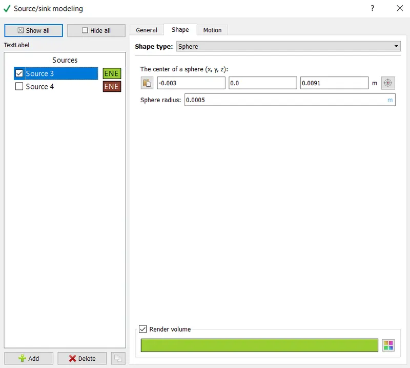
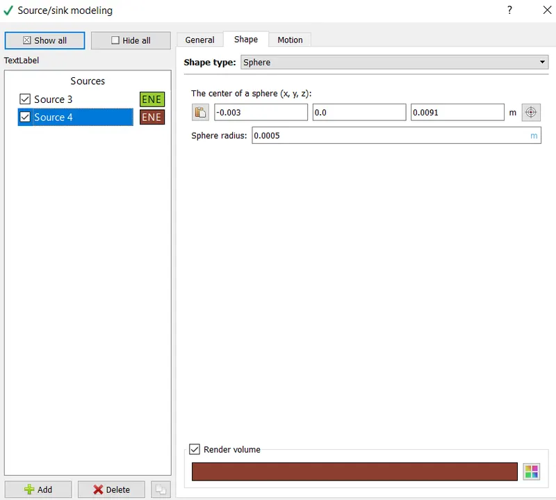
Shape tab> choose sphere

Radius: 0.0005m

Source2:

Energy: 0.02J

Mode: cyclic

Start: -15 degree

End: -5 degree

Duration: 720 degree

Shape tab> choose sphere

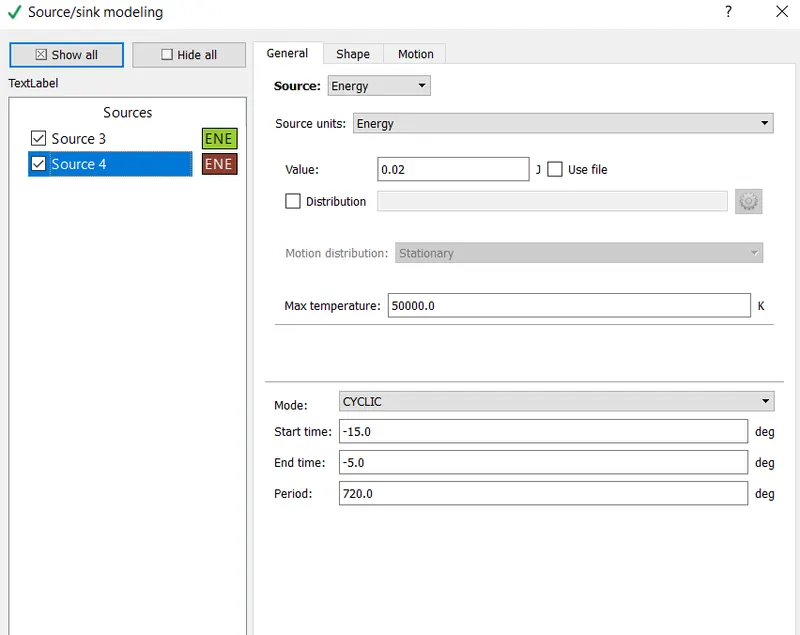
Radius: 0.0005m

Grid control:

Enable fixed embedding

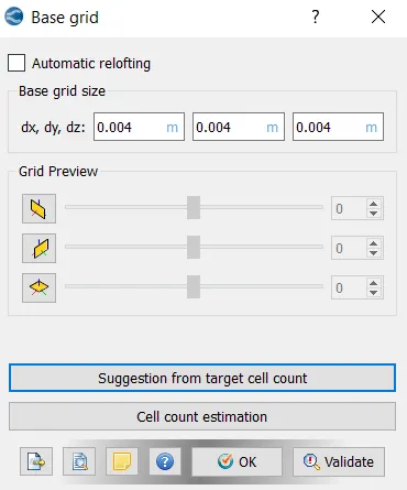
Base grid:

Choose base grid as 4mm

Fixed embedding:

Embedding is performed to refine the grid scale factor at different regions of geometry.

1. Intake valve and exhaust valve embedding

Fixed embedding are provided in the region of intake and exhaust valve angle regions as mesh size of 4mm will give inaccurate results.

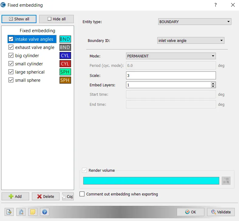
Intake valve angles

Entity type: boundary

Boundary ID- Intake valve angles

Mode- permanent

Scale- 3

Embedded layer- 1

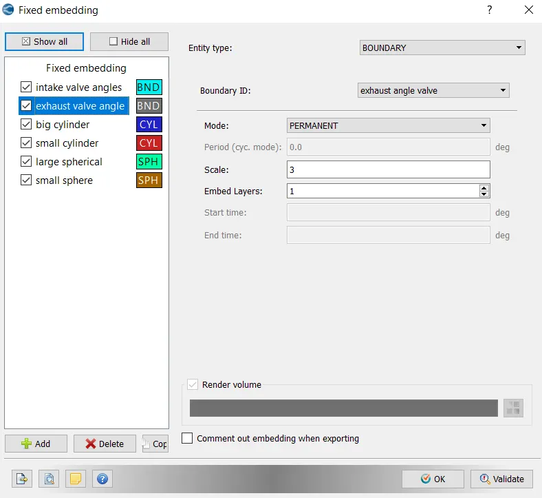
Exhaust valve angles

Entity type: boundary

Boundary ID- Exhaust valve angles

Mode- permanent

Scale- 3

Embedded layer- 1

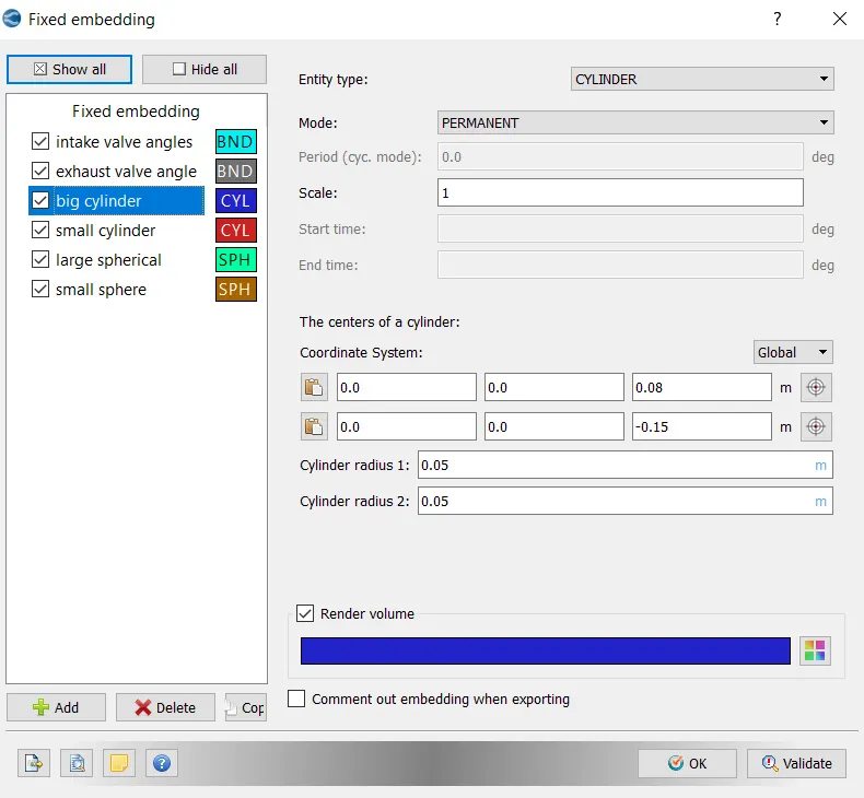
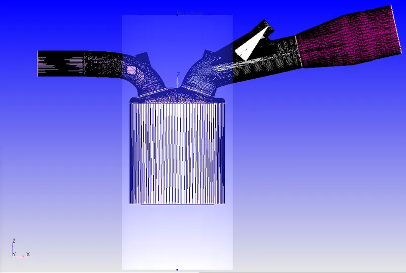
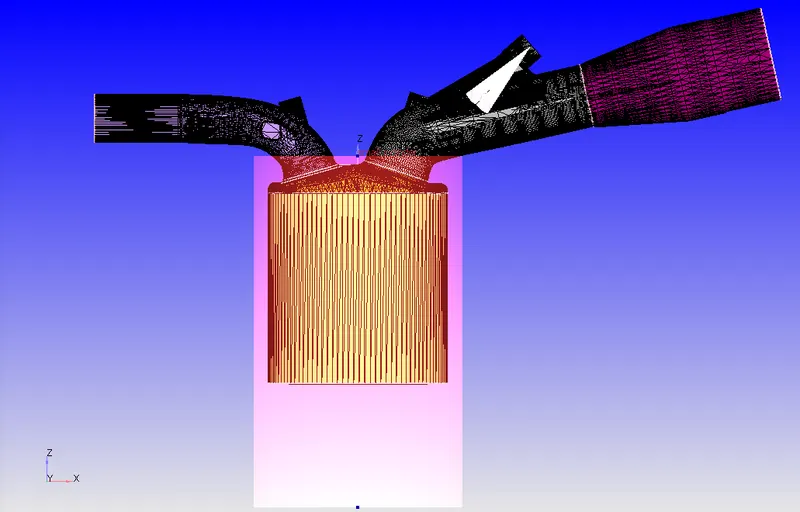
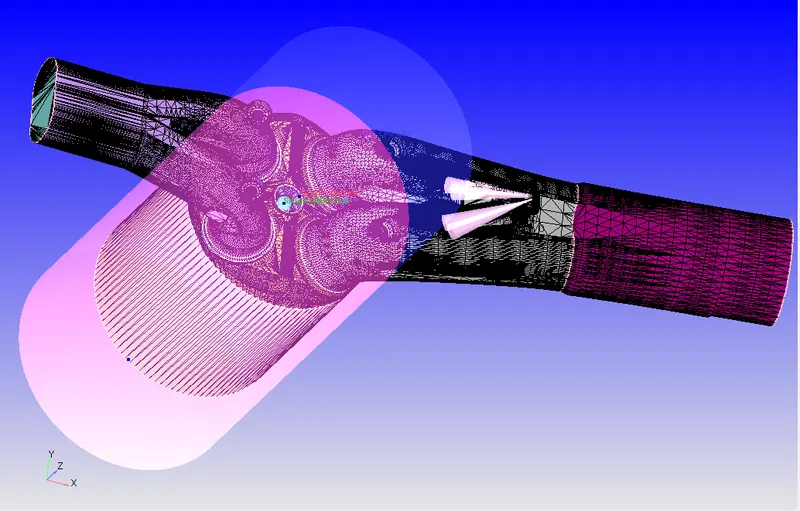
2. Big cylinder embedding

Entity type: cylinder

Mode- permanent

Scale- 1

Centre 1: (0, 0, 0.08)

Centre 2: (0, 0, -0.15)

Cylinder radius 1: 0.05m

Cylinder radius 2: 0.05m

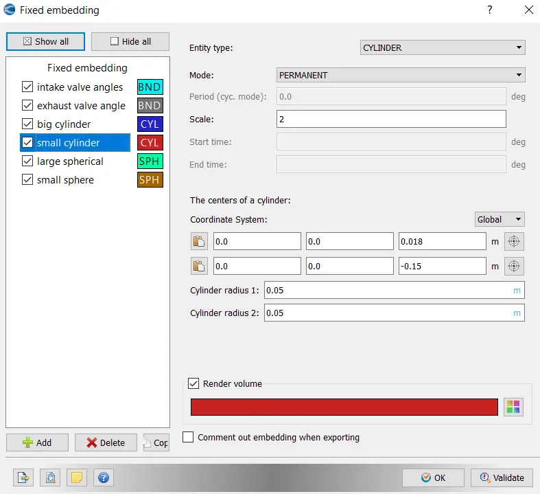
3. Small cylinder embedding

Entity type: cylinder

Mode- permanent

Scale- 2

Centre 1: (0, 0, 0.018)

Centre 2: (0, 0, -0.15)

Cylinder radius 1: 0.05m

Cylinder radius 2: 0.05m

Spherical embedding:

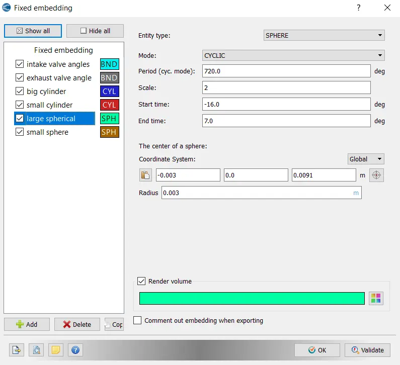
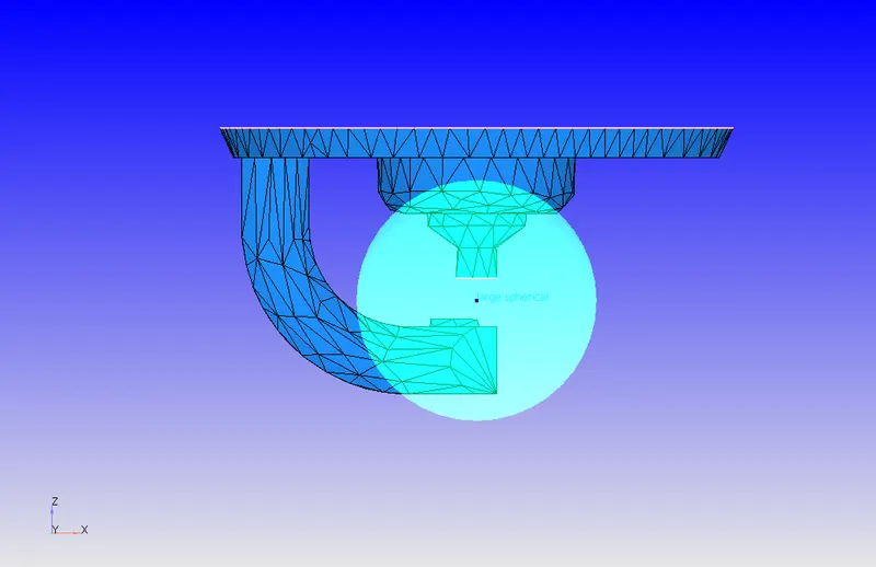
Spherical embedding is added on the region of source. Since during the initial time phase, there would be no combustion, so to initiate the combustion highly refined regions are to be created. We provide a larger embedding and a smaller embedding.

4. Large sphere

Entity: sphere

Mode: cyclic

Period: 720 degree

Start: -16 degree

End: 7 degree

Center location of sphere (-0.003, 0, 0.0091)

Radius: 0.003 m

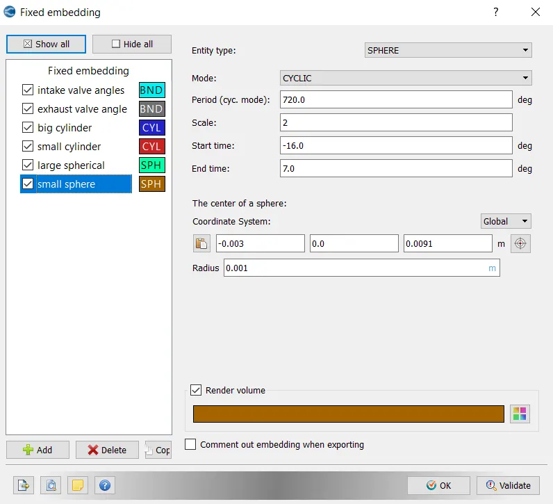
5. Small sphere

Entity: sphere

Mode: cyclic

Period: 720 degree

Start: -16 degree

End: 7 degree

Center location of sphere (-0.003, 0, 0.0091)

Radius: 0.001 m

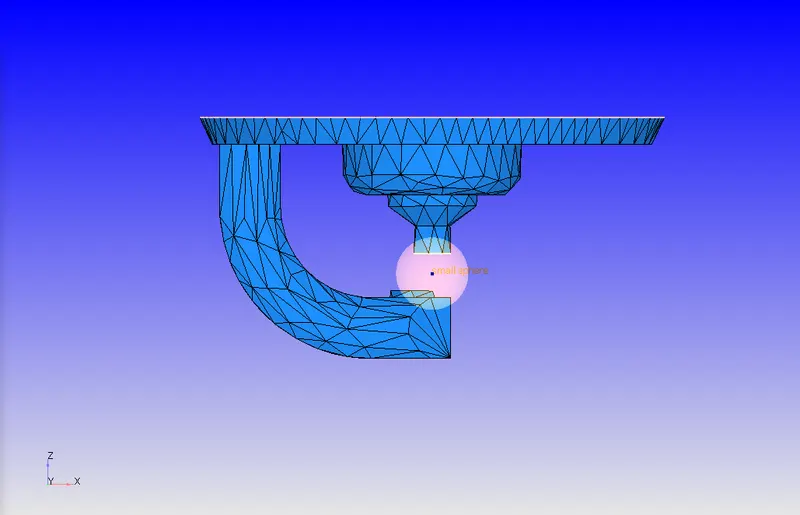
Final look at the PFI engine after total embedding

Adaptive mesh refinement (AMR):

Fixed embedding is preferred at the regions of complete boundary area. When refinement has to be done on the regions of flow equations, the refinement is called adaptive mesh refinement. Sub grid scaling approach is used to scale down the refinement of mesh.

For a scalar, the sub grid is defined as the difference between actual field and resolved field.

`∅^'=∅-∅ ̅`

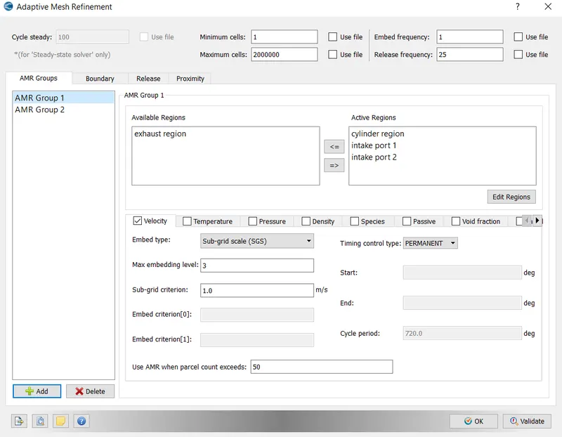
• Velocity AMR

The velocity AMR is kept constant, and is defined in the regions of cylinder, intake port 1 and intake port 2.

Minimum cells:1

Maximum cells:2e6

Timimg control: permanent

Embed type: SGS

Sub grid criteria:1

Maximum embed level:3

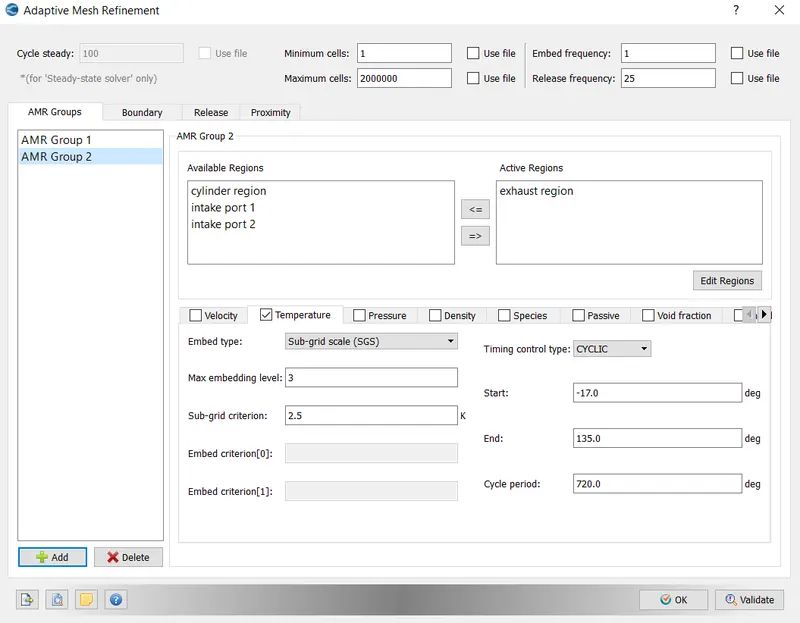
• Temperature AMR

The temperature AMR is defined in the exhaust region and is kept cyclic, since the exhaust moves during the opening and closing of valves.

Minimum cells:1

Maximum cells:2e6

Timimg control: cyclic

Embed type: SGS

Sub grid criteria:1

Maximum embed level:3

start:-17deg

End:135deg

Period:720deg

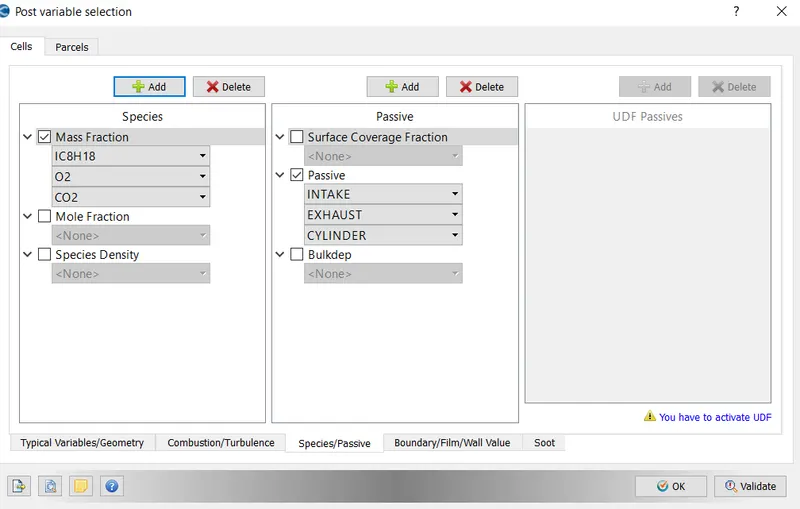
Post variable selection:

species: isooctane, o2, co2

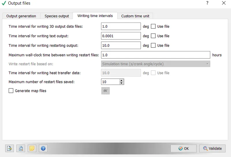
Output files:

Simulation run:

1. Export all the case set up from the converge studio
2. Go to Cygwin>> go to desired path or directory
3. Type the command mpiexec.exe -n 2 converge-intelmpi.exe restricted to run the simulation.

Post processing results and analysis:

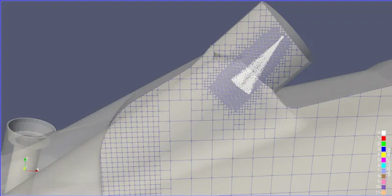
Mesh Refinement:

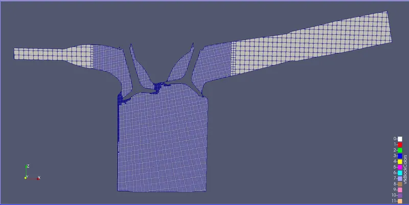
Mesh embeded refinement at injector section:

AMR animation:

In-cylinder pressure:

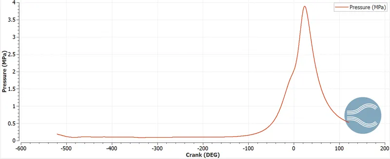
The in-cylinder pressure varies with crank angle at different strokes of cylinder. The pressure is highest at the end of compression stroke and decreases as the combustion and expansion takes place. At the end of compression stroke, the spark plug ignites the fuel, creating high cylinder pressure. At this high pressure, temperature is high enough to combust the fuel and the exhaust stroke moves down to release the pressure. The peak pressure reaches at 3.85MPa.

Animation:

In-cylinder volume:

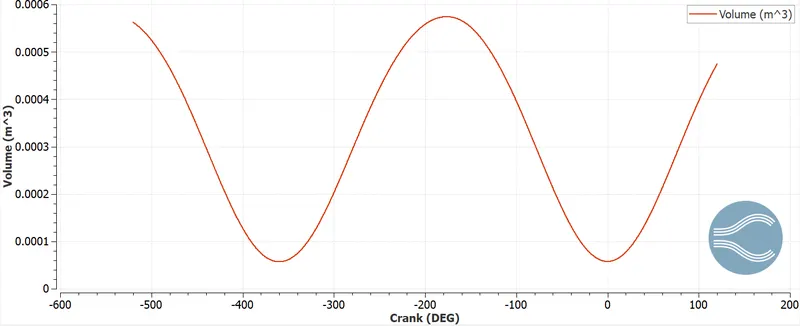
The volume variation with crank angle closely resembles the profile of a sine curve. The volume of the cylinder varies from TDC to BDC. The volume is minimum at TDC and maximum at BDC.

The compression ratio of the engine is the ratio of total volume to the clearance volume.

P-V plot:

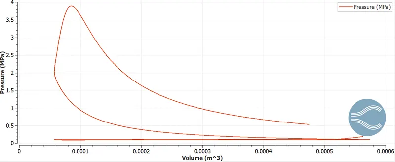
The P-V plot resembles Otto cycle diagram, and hence it shows how gasoline engine is based on this cycle. There are discontinuities in the graph because of the absence of exchange of working fluid and system at the original position.

From this PV diagram we can obtain the work done and power output from the engine.

The work done is given by the formula

`W=∫P dv`

Mean temperature:

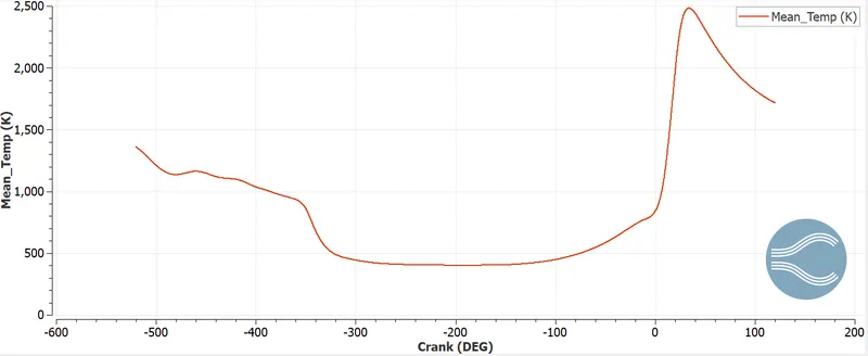
As the pressure varies inside the combustion chamber, so the temperature also varies. During the combustion, the peak temperature rise reaches 1700k and then reduces to 1300k at the exhaust phase. This data is extremely important for FEA engineers to determine the total thermal load pressure on this engine.

Animation:

IHR plot:

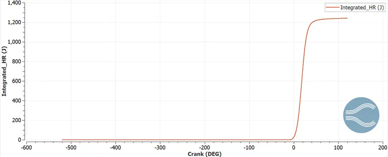
The mean temperature is maximum at the point when integrated heat release is close to maximum value i.e., entire heat energy is released. It is also the point of maximum pressure.

Density:

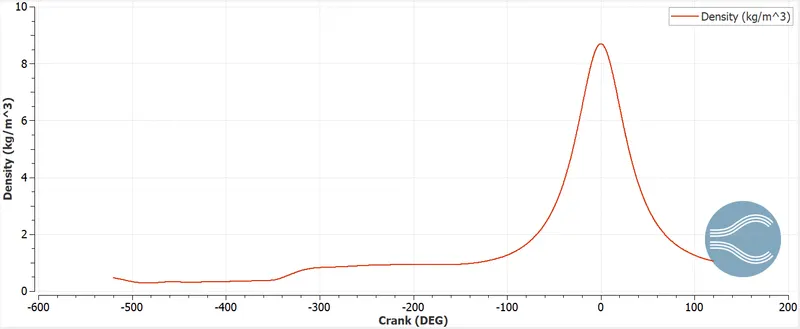
It is generally assumed that specific heat capacity remains constant, but practically they are all function of crank angle and they all depend upon temperature and pressure.

Mass:

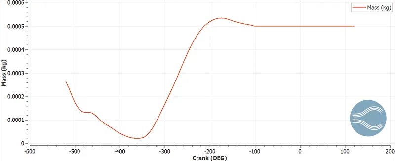
This plot tells us the amount of trapped mass inside combustion chamber. This data is important for the design engineers to modify the engine injector section in order to reduce the fuel mass from getting unburnt.

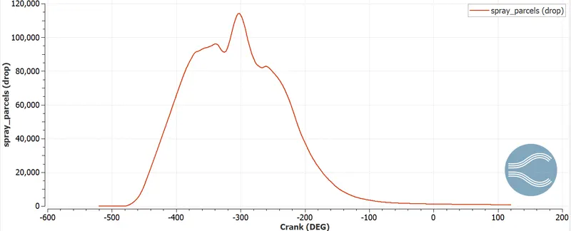
Spray parcel cylinder region:

The peak value touches 120000 parcels and further parcels drops down, this is because of the vaporization and combustion taking place. At the end almost zero parcels are seen which means there is not much fuel left over and less unburnt hydrocarbon.

Isobutane:

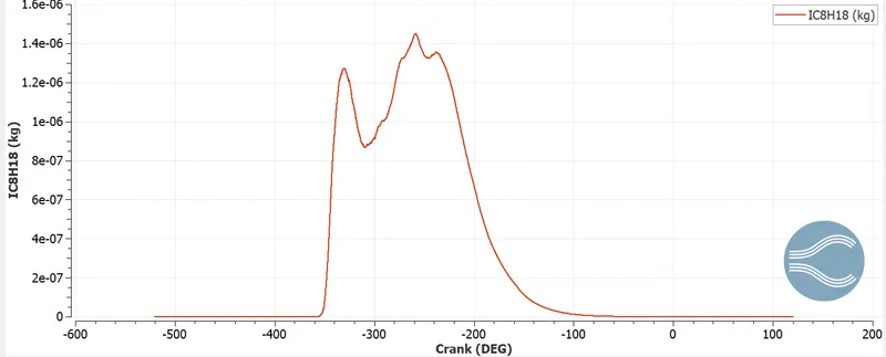
The fuel isobutane is observed to get vaporize more during the combustion period. This is because at peak temperature, more amount of fuel gets combusted to supply necessary power stroke. With the exhaust phase opening, the burning of the fuel mass decreases and reaches almost zero, confirming all fuel to get combusted with no trace of unburnt hydro carbon.

Animation:

Emission:

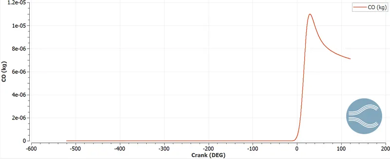
Undesirable emissions in IC engine is of major concern because of the negative impact on the environment and human health. Some undesirable emissions include unburnt hydrocarbons, soot, nox, so2 etc.

CO:

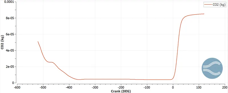
CO2:

Hiroy soot:

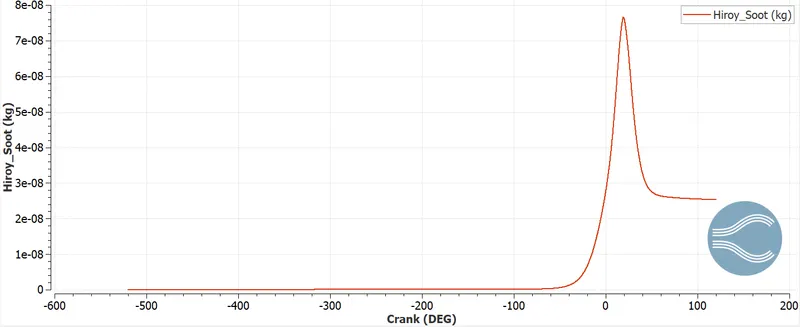
From the graphical data, it can be observed that soot formation is highest at the combustion phase with respect to crank angle. This is because all the reaction mechanism takes place at the combustion time and then reduces down. The maximum soot level is 7.8e-8 kg and the minimum level is 2.8e-8 kg. this predicts that design modifications are required to maintain the soot level as minimum as possible.

NOX plot:

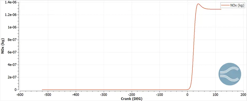
Nitrogen gets produced during the combustion reaction phase. Emission of nox is potentially harmful to human health. Before combustion the nox level is zero, since there are no reactions but gradually when the combustion starts the nox level increases. The maximum nox obtained is 9e-7 kg and then further reduces at the exhaust to 8.6e-7 kg.

HC:

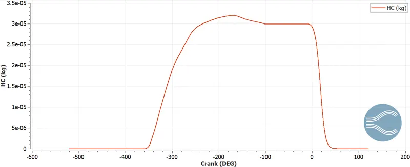
Unburnt hydrocarbon emission take place when the stoichiometric composition of fuel is richer than air. The unburnt carbon when mixes with insufficient oxygen results in unburnt hydrocarbon. The graphical data shows a maximum level of 3.3e-5kg of HC at the combustion period and then reduces to zero.

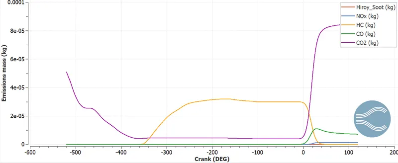
Comparison of emissions:

In a rich fuel mixture, there is not enough oxygen to react with all carbon and results in high level of HC and CO emissions. If the mixture is too lean, due to improper combustion can lead to HC emission.

From the graphical plot it can be seen that all emissions are at the peak level during the combustion period and drops down once the peak has reached.

What is the compression ratio of the engine?

The ratio of the maximum to minimum volume in the cylinder of an internal combustion engine is known as compression ratio.

`compression ratio=V_max/V_min =(0.0005625)/(5.70393e-5)=9.86513`

Combustion efficiency computation:

`combustion efficiency=(TOTAL HEAT RELEASE)/(TOTAL ENERGYCONTENT)`

The integrated heat release plot gives the amount of heat release during the combustion period. This data can be used to calculate the combustion efficiency by normalizing the energy content of fuel.

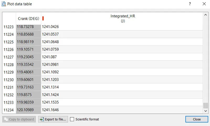
`TOTAL HEAT RELEASE=1241.1642 J`

`CALORIFIC VALUE OF GASOLINE= 44MJ/kg`

`Fuel mass per CYCLE=TOTALflow rate*time per 720 degree=(7.5e-4)*0.04=3e-5 kg`

`Total eENERGY content= CV*fuel mass per CYCLE=1320J`

`η_c=(IHR)/(TOTAL ENERGY CONTENT)=1241.1642/1320=94.02%`

The efficiency of the engine is 94.02%

Calculation of power and torque:

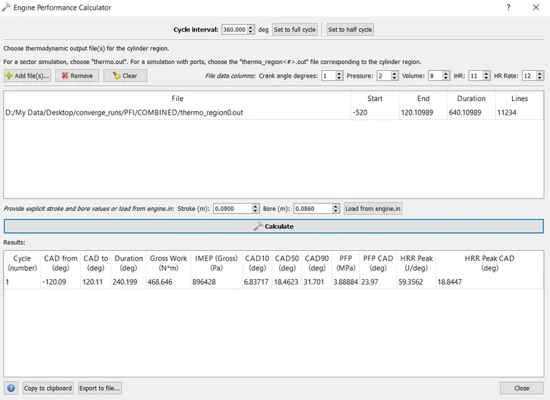
The work done of the engine is calculated from the engine performance calculator from converge. The thermo region 0 and the engine file is loaded in the engine performance calculator.

Go to line plotting module>select tools> select engine performance calculator> load thermo region 0.out file and engine file for bore and stroke values. Click on calculate.

`RPM=3000`

`RPS=3000/60=50`

`DPS=RPS*360=50*360=18000`

`TIME PER DEGREE=1/DPS=1/18000=5.55e-5`

`TIME PER 720 DEGREE=(5.55e-5)*720=0.04`

So, for one cycle of operation time taken= 5.55e-5*240.199=0.01331s

Power required,

`P=(WORKDONE)/(TIME TAKEN FOR ONE CYCLE OPERATION)=468.646/0.01331=35.5W`

Now for torque calculation

`T=(P*60)/(2*pi*N)=(35154.60*60)/(2*3.142*3000)=111.9Nm`

Though work done and torque has same units but the meanings are completely different.

Crank angle rotation at 10, 50 and 90 degree are given below:

CA 10: 6.83717deg

CA 50: 18.4623deg

CA 90: 31.701deg

Peak HRR: 59.3562 J

IMEP= 896428Pa

Why do we need a wall heat transfer model?

Internal combustion engines in today’s scenario are highly optimized in their performance. Experimental analysis performed to optimize thermodynamic model can increase computational cost and time. For high accuracy of engine performance prediction modelling of wall heat transfer and wall temperature are necessary.

For a better prediction of engine performance, heat transfer modelling from hot gas to engine parts, inside engine parts and also heat transfer to coolant and lubricating oil. Better heat transfer model can produce better emission prediction, performance and combustion parameters.

Heat transfer inside the combustion chamber takes place in all modes. When heat transfer takes place in multiple mode, conjugate heat transfer is applied. Simulating IC engine flow along with conjugate heat transfer increases the computational time. So in case of cylinder wall heat transfer different models are used to predict the CFD simulation.

Why can’t we predict the wall temperature from the CFD simulation?

In general IC engine combustion is based on chemical reaction. During the combustion phase, the fuel-air gets mixes up and gets ignited by the spark plug. These chemical reaction raises the temperature inside the combustion chamber and the piston becomes free to expand. The heat transfer between the solid and fluid takes place in two modes- convection and radiation. In case of fluid flow, Navier-Stokes equations are solved. To get accurate results finer mesh sizes are considered.

For the present case PFI engine simulation, the computation takes a lot of time to solve the complex geometry and processes. So for conjugate heat transfer, the solid cylinder wall is solved by super cycling process and fluid domain is solved by transient case. Now for the fluid domain, the computational time takes a lot because at each cell volume, the Navier Stokes equations are solved. So certain physical models are used to approximate the computational time. Wall heat transfer model are focused on heat transfer rather than fluid simulation.

What is the significance of CA 10, 50 and 90?

The CA refers to crank angle followed by its position in a degree at 10%, 50% and 90% of combustion. These angles are captured to store data such as heat release, combustion data. The significance of CA 10 determines the start of ignition, CA 50 determines the end of premixed combustion and CA 90 determines the burning of unburnt fuel inside combustion. These data are essential to compare the simulation results with the experimental outcomes, or the simulation data from the previous results at specified percentage.

Conclusions:

1. The hydro simulation has run successfully to operate the combustion process and measure performance parameters.
2. Refinement of mesh using fixed embedding and adaptive mesh refinement technique has been applied at different zones of interest. A finer mesh yields best computational results.
3. Performance calculator has been utilised to capture the work done during one cycle of simulation. Combustion efficiency, compression ratio, torque and power calculation has been performed to measure overall performance level of PFI engine.
4. Spray modelling and RNG k-epsilon turbulent model has been applied to get a better combustion model from post processing analysis.