Shock tube simulation using CONVERGE cfd

Abstract:

Shock tubes are used for investigating compressible flows and study gas phase combustion problems. In this problem, a shock tube chamber is setup filled with air at two different pressure zones, with a diaphragm in the middle. Study of shock wave propagation along with its effect on temperature, pressure and velocity is analysed completely.

Introduction:

The shock tube is an instrument used to replicate and direct blast waves at a sensor or a model in order to simulate actual explosions and their effects, usually on a smaller scale. Shock tubes (and related impulse facilities such as shock tunnels, expansion tubes, and expansion tunnels) can also be used to study aerodynamic flow under a wide range of temperatures and pressures that are difficult to obtain in other types of testing facilities. Shock tubes are also used to investigate compressible flow phenomena and gas phase combustion reactions. More recently, shock tubes have been used in biomedical research to study how biological specimens are affected by blast waves.

A simple shock tube is a tube, rectangular or circular in cross-section, usually constructed of metal, in which a gas at low pressure and a gas at high pressure are separated using some form of diaphragm. The diaphragm suddenly bursts open under predetermined conditions to produce a wave propagating through the low pressure section. The shock that eventually forms increases the temperature and pressure of the test gas and induces a flow in the direction of the shock wave. Observations can be made in the flow behind the incident front or take advantage of the longer testing times and vastly enhanced pressures and temperatures behind the reflected wave.

The low-pressure gas, referred to as the driven gas, is subjected to the shock wave. The high pressure gas is known as the driver gas. The corresponding sections of the tube are likewise called the driver and driven sections. The driver gas is usually chosen to have a low molecular weight, (e.g., helium or hydrogen) for safety reasons, with high speed of sound, but may be slightly diluted to 'tailor' interface conditions across the shock. To obtain the strongest shocks the pressure of the driven gas is well below atmospheric pressure (a partial vacuum is induced in the driven section before detonation).

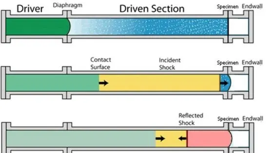
The test begins with the bursting of the diaphragm. Several methods are commonly used to burst the diaphragm.

1. A mechanically-driven plunger is sometimes used to pierce it or an explosive charge may be used to burst it.
2. Another method is to use diaphragms of plastic or metals to define specific bursting pressures. Plastics are used for the lowest burst pressures, aluminium and copper for somewhat higher levels and mild steel and stainless steel for the highest burst pressures. These diaphragms are frequently scored in a cross-shaped pattern to a calibrated depth to ensure that they rupture evenly, contouring the petals so that the full section of the tube remains open during the test time.
3. Yet another method of rupturing the diaphragm utilizes a mixture of combustible gases, with an initiator designed to produce a detonation within it, producing a sudden and sharp increase in what may or may not be a pressurized driver. This blast wave increases the temperature and pressure of the driven gas and induces a flow in the direction of the shock wave but at lower velocity than the lead wave.

The bursting diaphragm produces a series of pressure waves, each increasing the speed of sound behind them, so that they compress into a shock propagating through the driven gas. This shock wave increases the temperature and pressure of the driven gas and induces a flow in the direction of the shock wave but at lower velocity than the lead wave. Simultaneously, a rarefaction wave, often referred to as the Prandtl-Meyer wave, travels back in to the driver gas.

Objective:

• Setup a transient shock tube simulation
• Plot the pressure and temperature history in the entire domain - Explain the result
• Plot the cell count as a function of time - Explain the result

Geometrical preparation:

Open the Converge studio panel.

Drag and drop the shock tube .stl model format.

First we need to delete the partition edge corresponding to geometry from both the sides of pressure region

Go to repair>> select delete>enable triangle selection>select the entity and delete it.

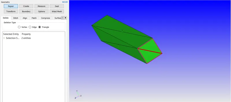
Repeat the same step for the other side of pressure region also

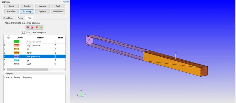
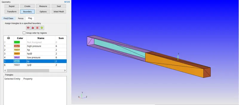
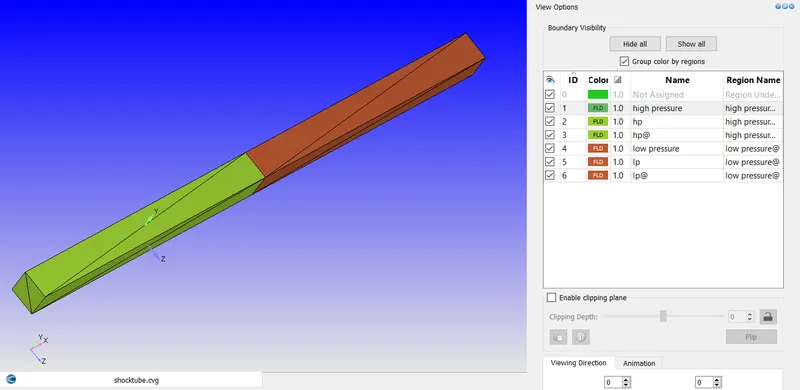
boundary flag:

high pressure

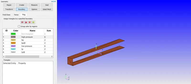
hp

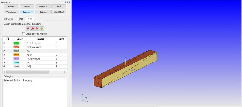
hp@

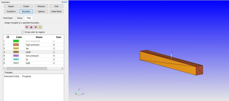
low pressure

lp

lp@

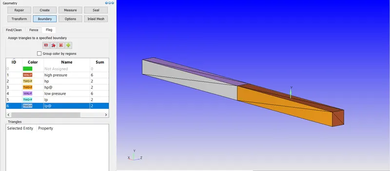
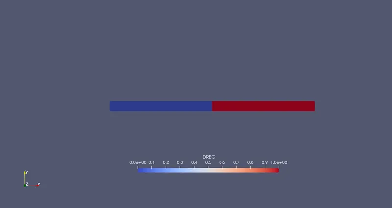
Now we group all the boundaries to region, so that we can identify seperately the high pressure region and low pressure region

go to view option>> select group color by region

Simulation case setup:

Open the converge studio panel

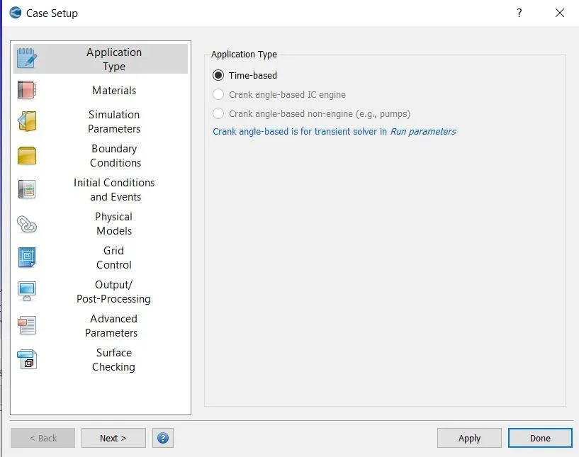
Application type: time based

Materials:

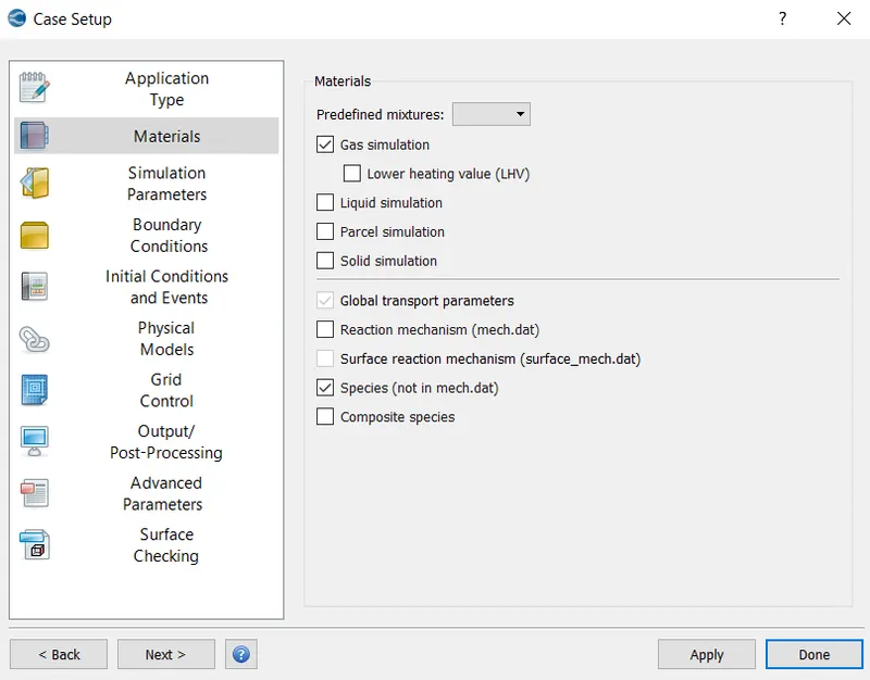
Predefined mixture: air

Enable the species option and disable the reaction mechanism file

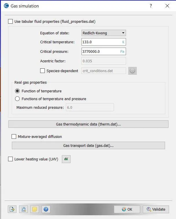
Gas simulation:

Select default parameter settings

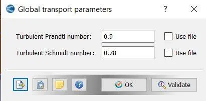
Global transport:

Select default settings

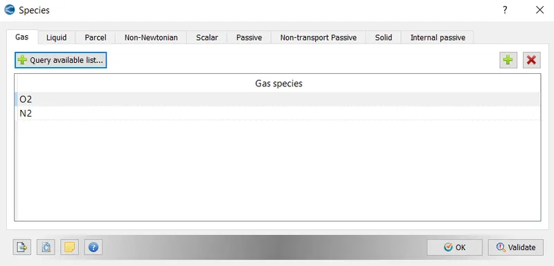
Species:

Add N2 and O2

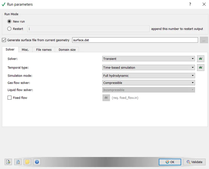
Simulation parameters:

Solver type: transient

Simulation mode: full hydrodynamic

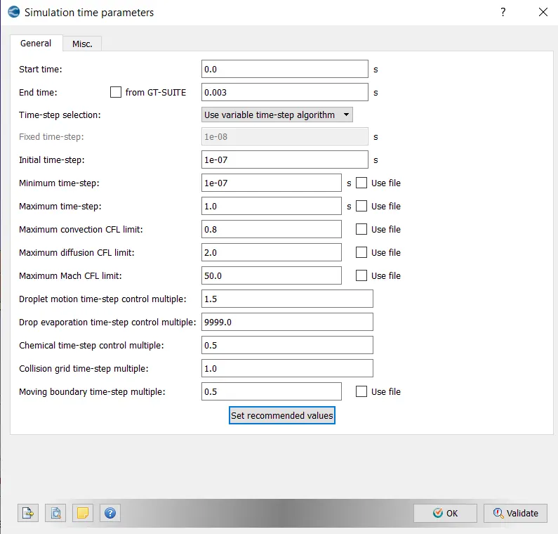
Simulation time parameter:

Start time 0s

End time 0.003s

Initial time step 1e-7

Minimum time step 1e-7

Maximum time step 1

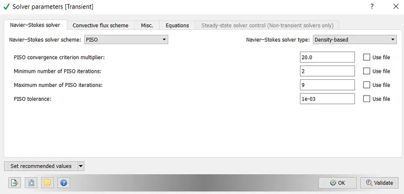
Solver parameter:

Navier Stokes equation solver: density

Boundary conditions:

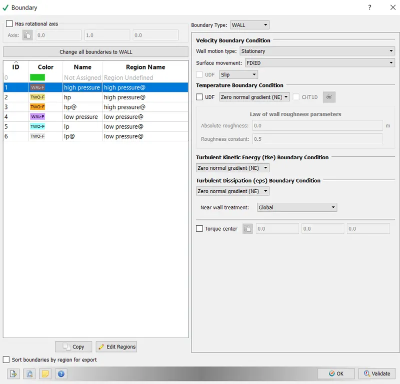
High pressure

Boundary type: wall

Wall motion type: stationary, slip

Region name: high pressure

Temperature: zero normal gradient

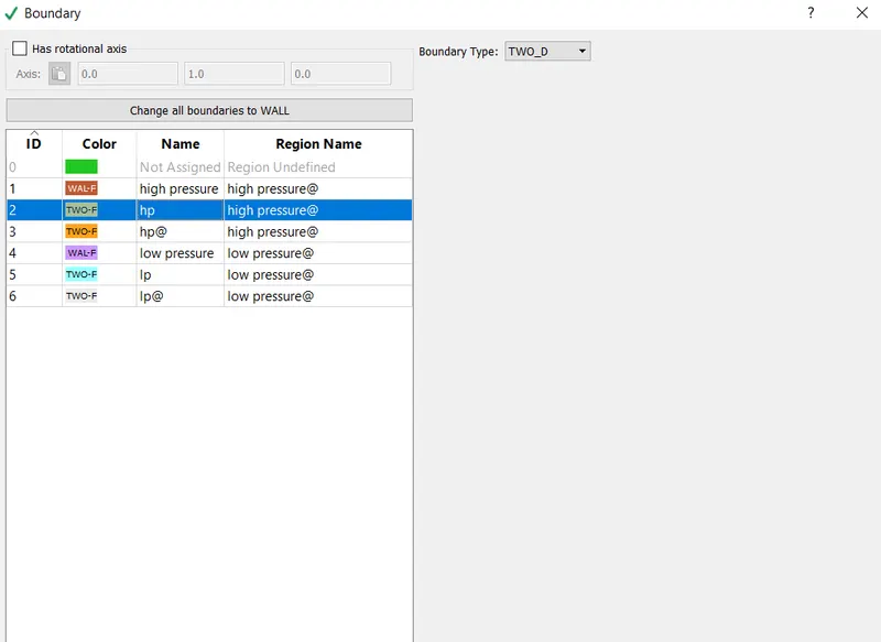
Hp

Boundary type: 2D

Region name: high pressure

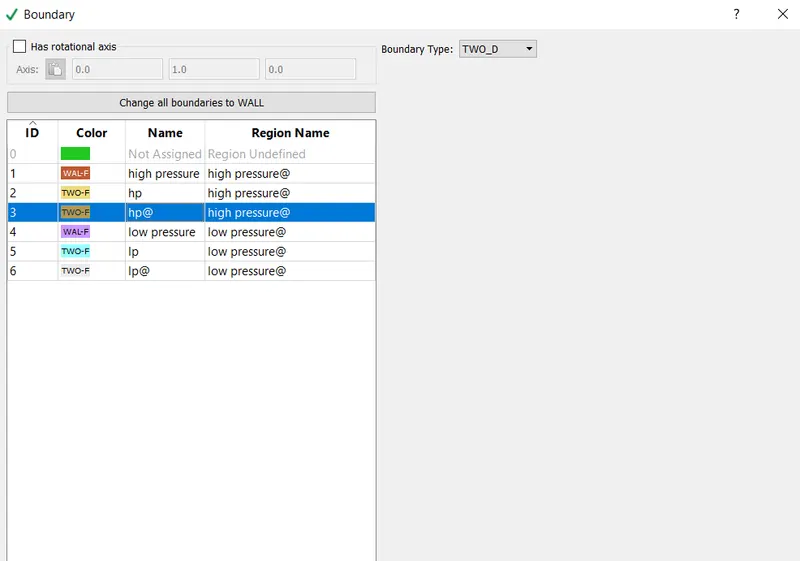
hp@

boundary type: 2D

Region name: high pressure

low pressure

Boundary type: wall

Wall motion type: stationary, slip

Region name: low pressure

Temperature: zero normal gradient

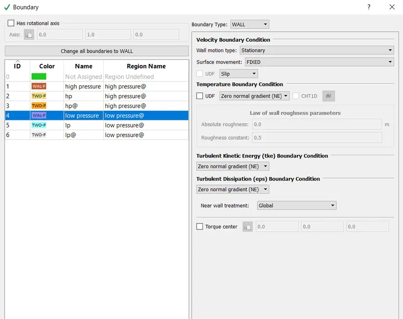
lp

Boundary type: 2D

Region name: low pressure

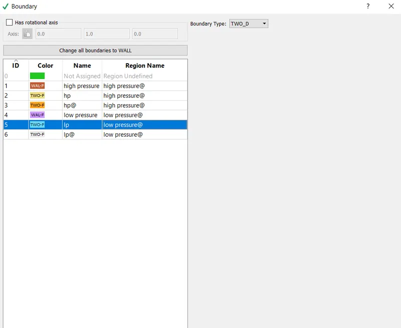
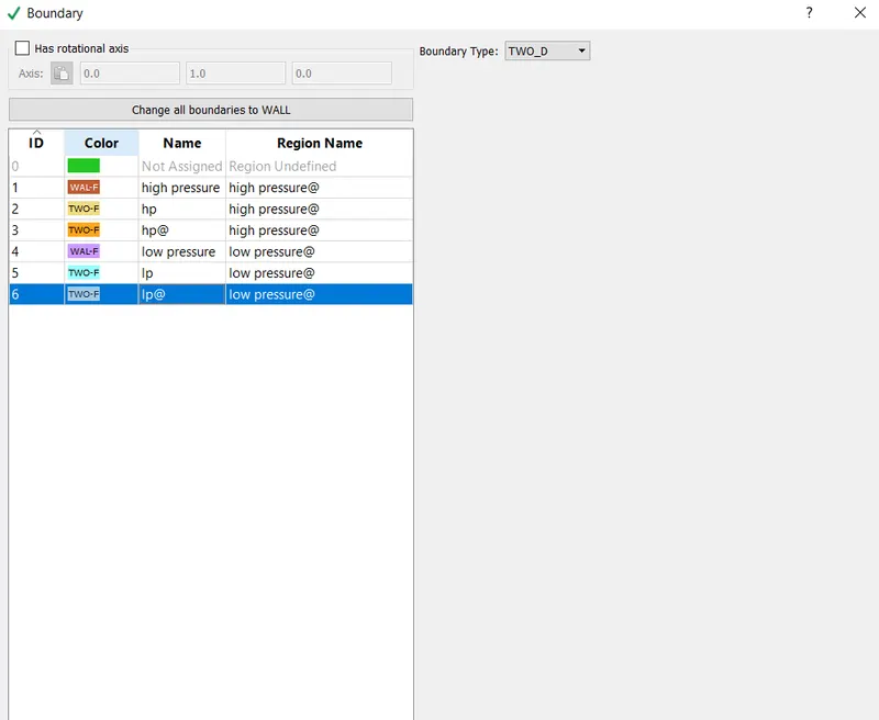
lp@

boundary type: 2D

Region name: low pressure

Initial condition and events:

Enable the event check box

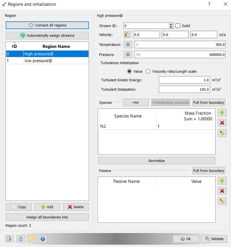
Region name: high pressure@

REGION ID-0

Velocity 300m/s

Pressure: 6e5Pa

Species: N2

Mass fraction 1

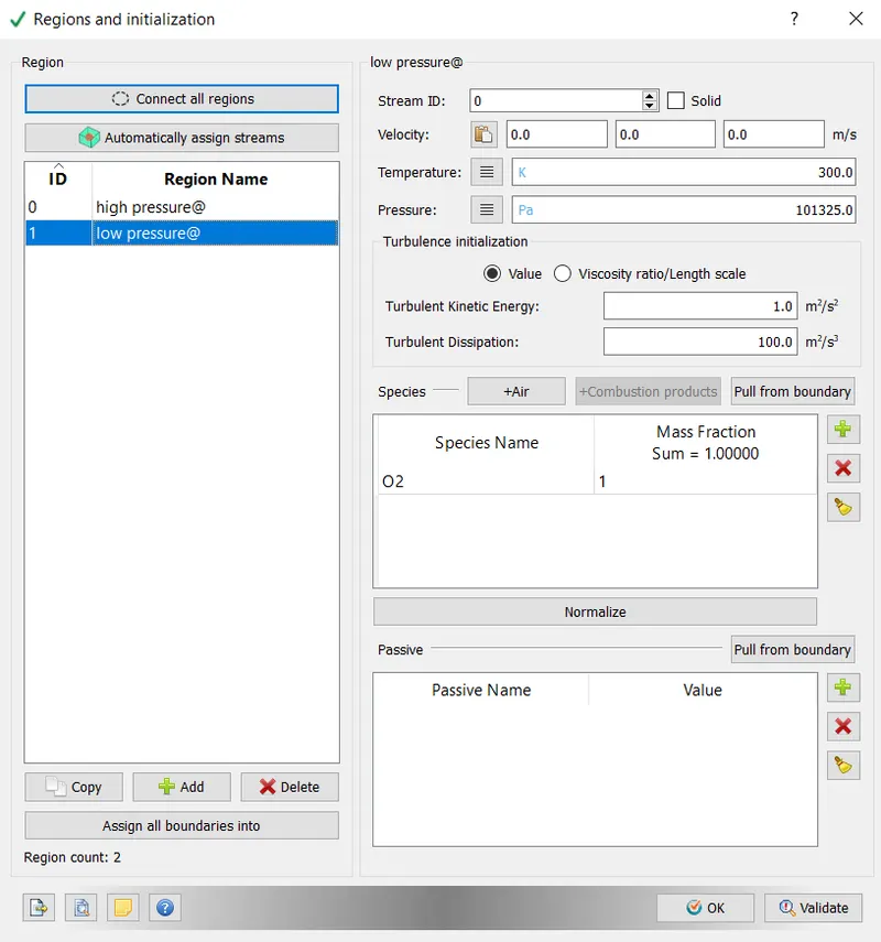
Region name: low pressure@

REGION ID-0

Velocity 300m/s

Pressure: 101325Pa

Species: O2

Mass fraction 1

Events

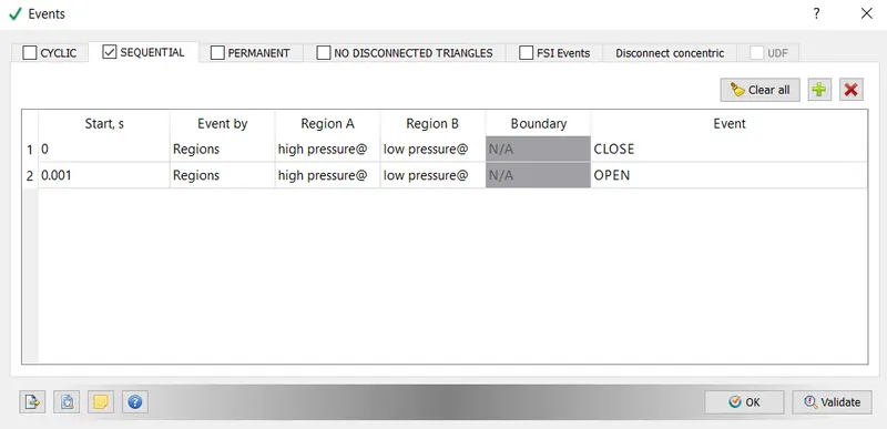
Click on events>> select sequential>> choose region A as high pressure@ and region B as low pressure@

For start time 0, choose event as close

For start time 0.001s, choose event as open

Physical model

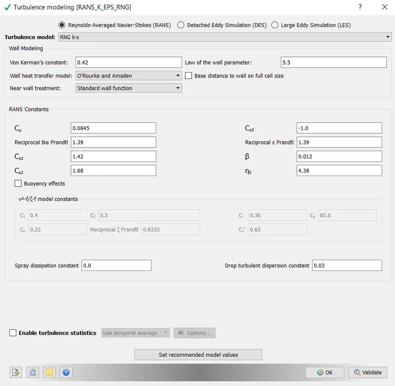
Choose RNG K-epsilon model

Grid control:

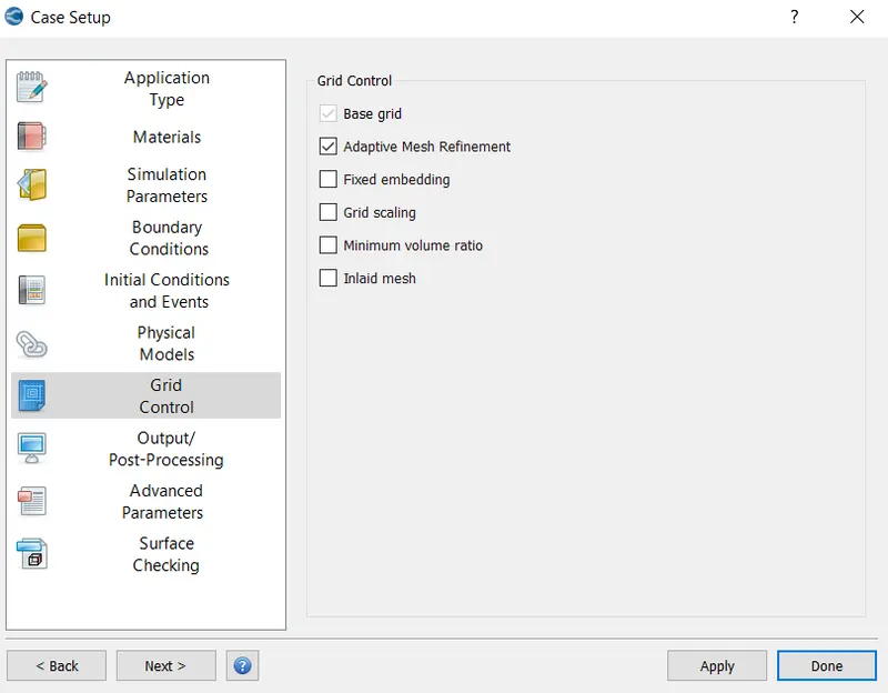
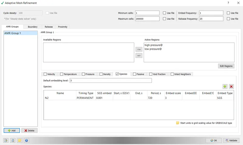
Select the option of adaptive mesh refinement

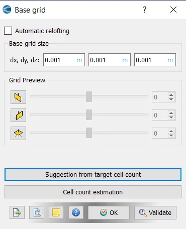
Base grid: give base size of 0.001m

Adaptive mesh refinement:

Select species option

Min cells 0

Maximum cells: 200000

Active region: high pressure@, low pressure@

Species name: N2

Timing type permanent

SGS embedding 0.001

Period 720 embeded scale 3

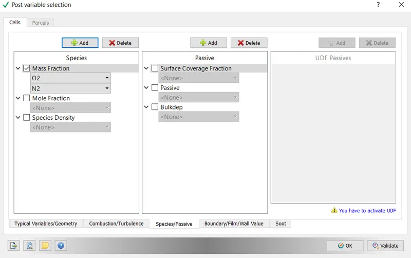
Post variable selection:

Go to species>> choose mass fraction of N2 and O2

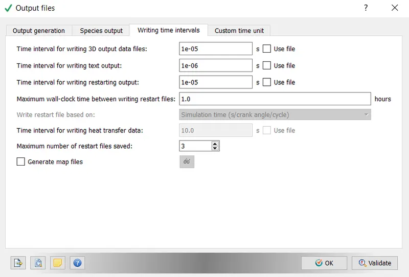
Output files:

Time interval for writing 3D output file 1e-5

Simulation run:

1. Export all the case set up from the converge studio
2. Go to Cygwin>> go to desired path or directory
3. Type the command mpiexec.exe -n 2 converge-intelmpi.exe to run the simulation.

Post processing analysis:

Graphical analysis

Pressure:

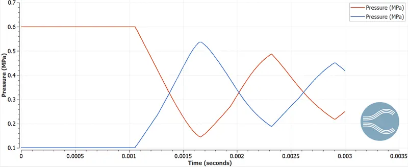
The high pressure region is at 0.6MPa. From 0.001s the diaphragm breaks and the high pressure region flows towards the low pressure region side by pushing. Due to this movement, density change takes place and the low pressure tends to resist the flow of high pressure flow. This ongoing pressure fluctuation gives rise to shock waves propagating forward producing compression and rarefaction waves. Due to shock, a sinusoidal drop in pressure is noted from high pressure to low pressure zone and vice versa.

Mean temp:

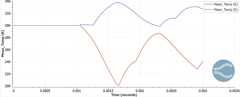
From the graph, at time 0.001s the partition breaks and the shock wave start to propagate. The zone of high pressure has temperature rising up initially and then starts decreasing. This is because of reflection of shock waves. As a pressure from high pressure zone moves towards the low pressure, the peak magnitude of temperature dropping. This also indicates the reduction of shock wave.

Cell count:

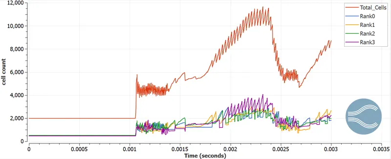
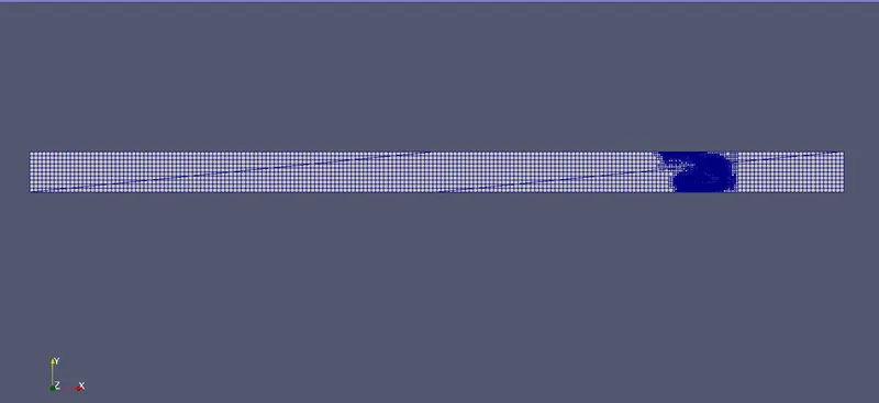
Total cell count shows the variation of mesh sizes as a function of time during the time of simulation run. In the event settings has been done for the diaphragm to burst at 0.001s and as a result of this certain peak spikes in cell count is seen. When simulation starts the high pressure region pushes the low pressure region and the AMR gets activated. The sudden decrease in the cell count is when the reflected pressure pushes back.

ID REGION

Mesh:

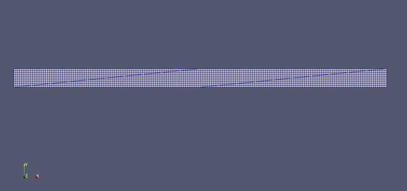
Mesh with AMR effect:

Velocity contour:

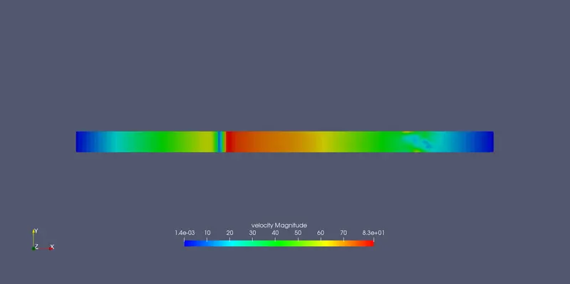
The velocity contour represents the magnitude with which the shock propagates inside the tube. The maximum velocity of 8.3e1 m/s is located at the mid-section where the diaphragm is ruptured. Mini shock waves are generated, and after several reflection and rarefaction minimum velocity point is found at the corner and maximum at the middle.

Animation:

Temperature contour:

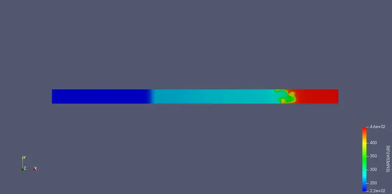
At the breakage of diaphragm, temperature fluctuation starts due to shock wave generation. The reflected shock wave generates more temperature and pressure increment. The maximum temperature remains at the zone of high-pressure region, where shock waves hits and keeps dropping in magnitude.

Animation:

Pressure contour:

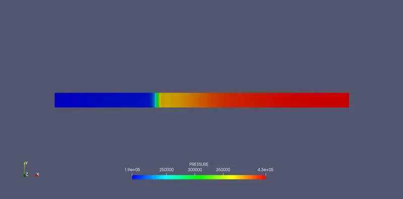
At the rupture of diaphragm, shock waves gets generated. The shock wave captured is elliptic in shape. At the location of shock, pressure in N2 decreases whereas for O2 region it increases. The pressure wave gets reflected continuously and drops, so that the intensity of shock reduces.

Animation:

Mass fraction of N2

Mass fraction of O2

Conclusions:

1. The burst of diaphragm enables to capture the velocity, temperature and pressure distribution due to shock wave.
2. The pressure gradient between the driver and the driven section is due to the viscous drag and friction between the shock wavefront and shock tube wall.
3. For combustion simulation, shock tubes are made to auto ignite the fuel without any external mechanism.