Steady state simulation of flow over a throttle body using CONVERGE CFD

Abstract:

In this project, a steady state simulation of throttle valve is studied using CONVERGE cfd. Pressure based solver with RNG k-epsilon turbulent model is used for simulation. Parameters like mass flow rate, velocity distribution, pressure variation across the throttle region is observed and analyzed. Embedded scaling is done to refine the mesh at the throttle interface and capture the physics of flow accurately.

Aim:

Steady state simulation over a throttle body

Objective:

1. Set up and run the steady state simulation for flow over throttle body.
2. Post process the results and show pressure and velocity contours.
3. Show the mesh (i.e surface with edges)
4. Show the plots for pressure, velocity, mass flow rate and total cell count.
5. Create an animation in which it throttle movement should be visible.

Introduction:

A throttle is the mechanism by which fluid flow is managed by constriction or obstruction.

In an IC engine the throttle is a means of controlling an engine's power by regulating the amount of fuel or air entering the engine. In a motor vehicle the control used by the driver to regulate power is sometimes called the throttle, accelerator, or gas pedal. For a gasoline engine, the throttle most commonly regulates the amount of air and fuel allowed to enter the engine. Recently, for a GDI engine, the throttle regulates the amount of air allowed to enter the engine. The throttle of a diesel, when present, regulates the air flow into the engine.

Historically, the throttle pedal or lever acts via a direct mechanical linkage. The butterfly valve of the throttle is operated by means of an arm piece, loaded by a spring. This arm is usually directly linked to the accelerator cable, and operates in accordance with the driver, who hits it. The further the pedal is pushed, the wider the throttle valve opens.

Modern engines of both types (gas and diesel) are commonly drive by wire systems where sensors monitor the driver controls and in response a computerized system controls the flow of fuel and air. This means that the operator does not have direct control over the flow of fuel and air; the electronic control unit (ECU) can achieve better control in order to reduce emissions, maximize performance and adjust the engine idle to make a cold engine warm up faster or to account for eventual additional engine loads such as running air conditioning compressors in order to avoid engine stalls.

The throttle on a gasoline engine is typically a butterfly valve. In a fuel injected engine, the throttle valve is placed on the entrance of the intake manifold, or housed in the throttle body. In a carbureted engine, it is found in the carburetor. When a throttle is wide open, the intake manifold is usually at ambient atmospheric pressure. When the throttle is partially closed, a vaccuum develops as the intake drops below ambient pressure.

Simulation Case setup:

1. Open converge studio console
2. Drag and drop the throttle valve model in graphics panel.
3. To ensure better flow simulation, we delete the outer covering of the elbow wall>> select triangle entity selection>> choose angle mode>> select the outer elbow wall>> select delete
4. 
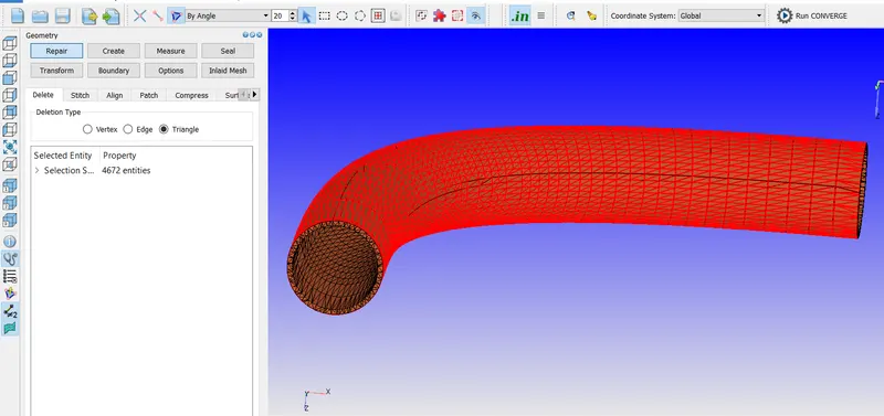
5. Follow the similar procedure for the inlet and outlet section as given in step 3.
6. 
7. 
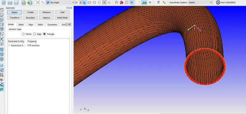
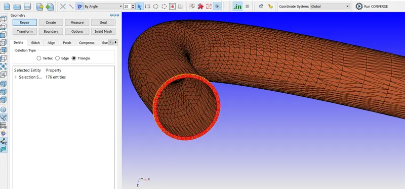
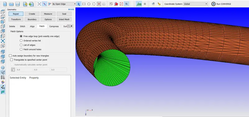
8. The inlet and outlet section are open and will generate open edge error.
9. To remove the error we provide patching>> select edge tab>> select open edge mode>> go to repair section>> select the inlet and outlet edge>> select patch and the apply. The openings will get closed.
10. 
11. 
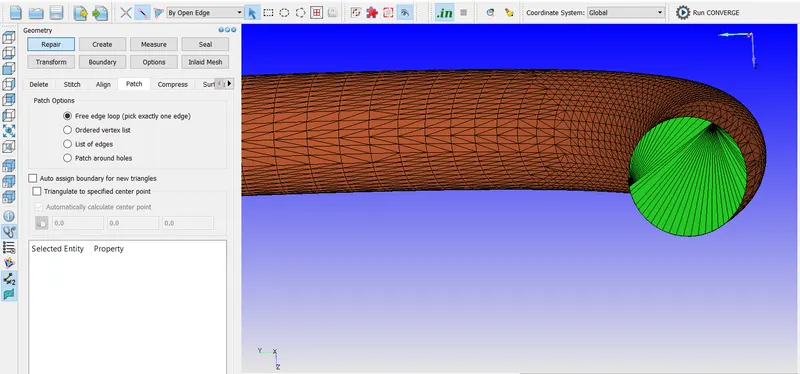
12. Go to option>> select bounding box. The dimension of the box will be highlighted>> change the scale to 0.001 in order to convert to meters.
13. The geometry is now created.
14. 
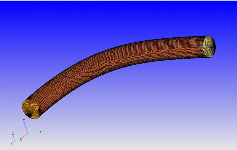
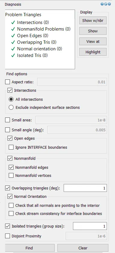
15. We conduct a diagnosis check to remove all the geometrical errors
16. 
17. Go to the right-hand side case set up option, there we will find many setting up option.
18. 
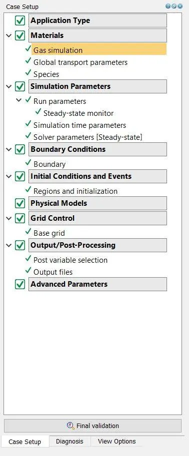
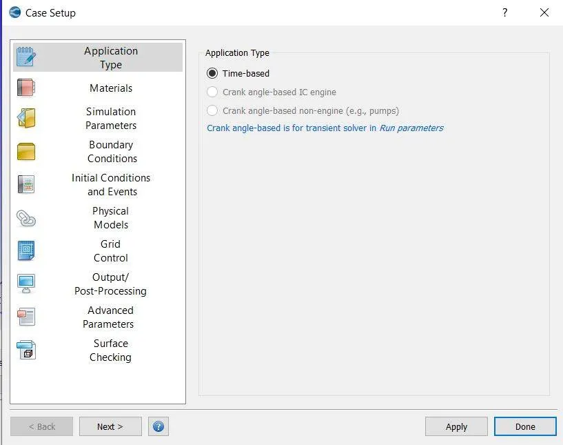
19. Select application option>>select time based option.
20. 
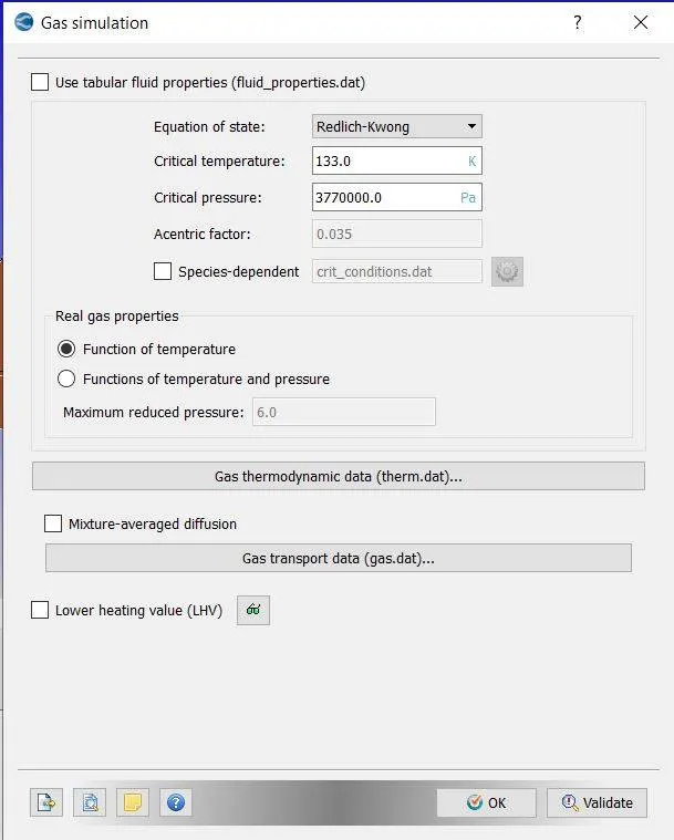
21. Go to materials>> select gas simulation >> click ok
22. 
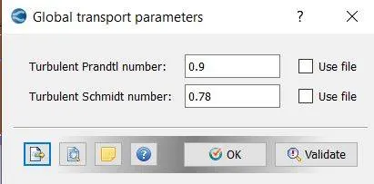
23. Go to global transport parameters >> select ok.
24. 
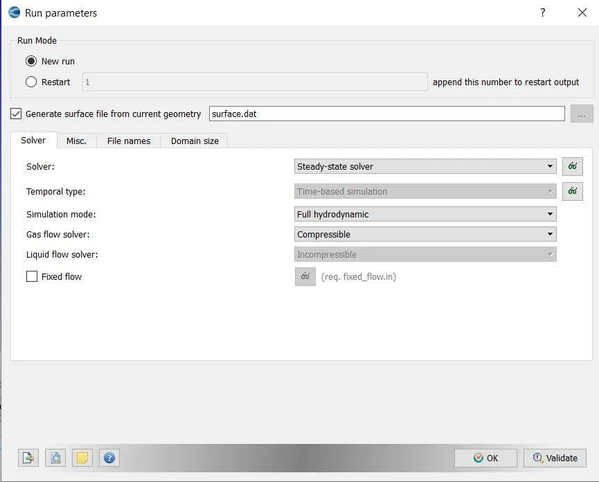
25. Go to simulation parameters>> select run parameters>> choose steady state solver with full hydrodynamic case.
26. 
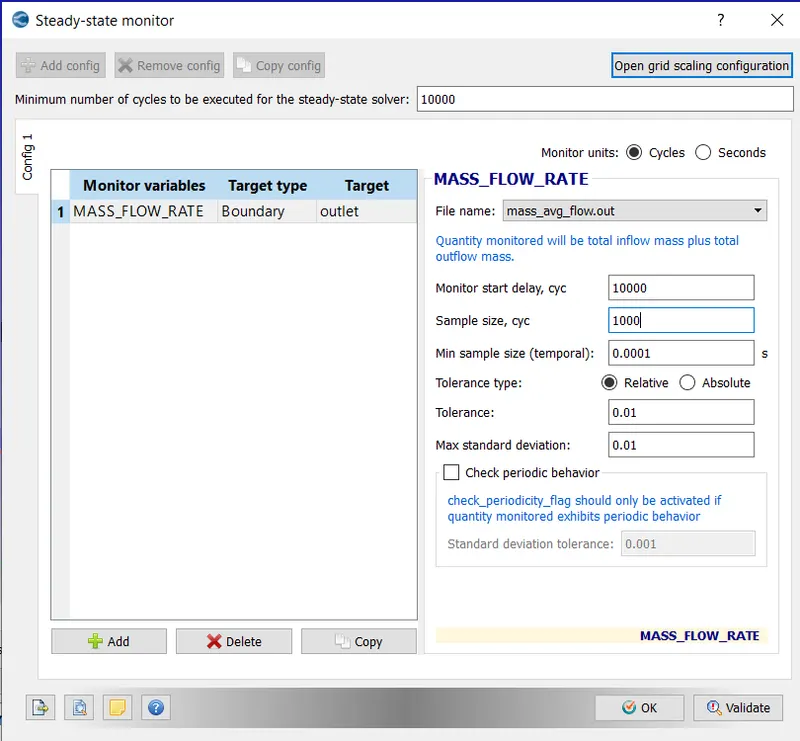
27. Go to steady state monitor>> provide monitor variable as mass flow rate>> select target type boundary>> select target as outlet
28. Provide the min no of cycles for steady state solver>> provide monitor delay start, sample size.
29. 
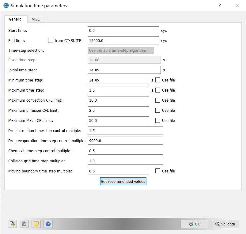
30. Select simulation time parameter>>provide end time as 15000 cycles>> provide initial and min time step of 1e-9 and max time step of 1
31. 
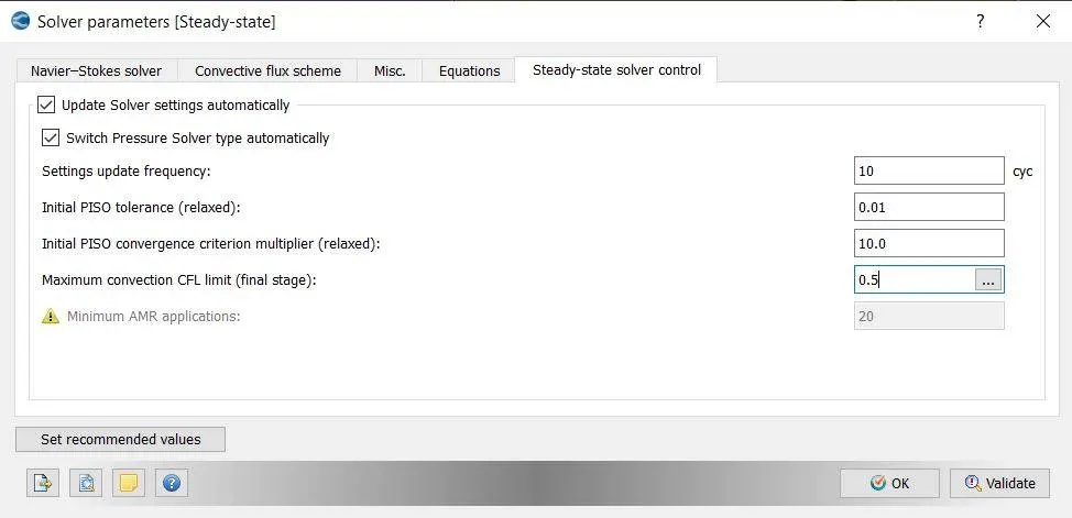
32. Go to solver parameter setting>> choose density based >> go to equation >>select pressure and set precondition to none>> go to solver control and define the cfl limit to 0.5
33. 
34. Go to boundary>> define all boundary region name with ID
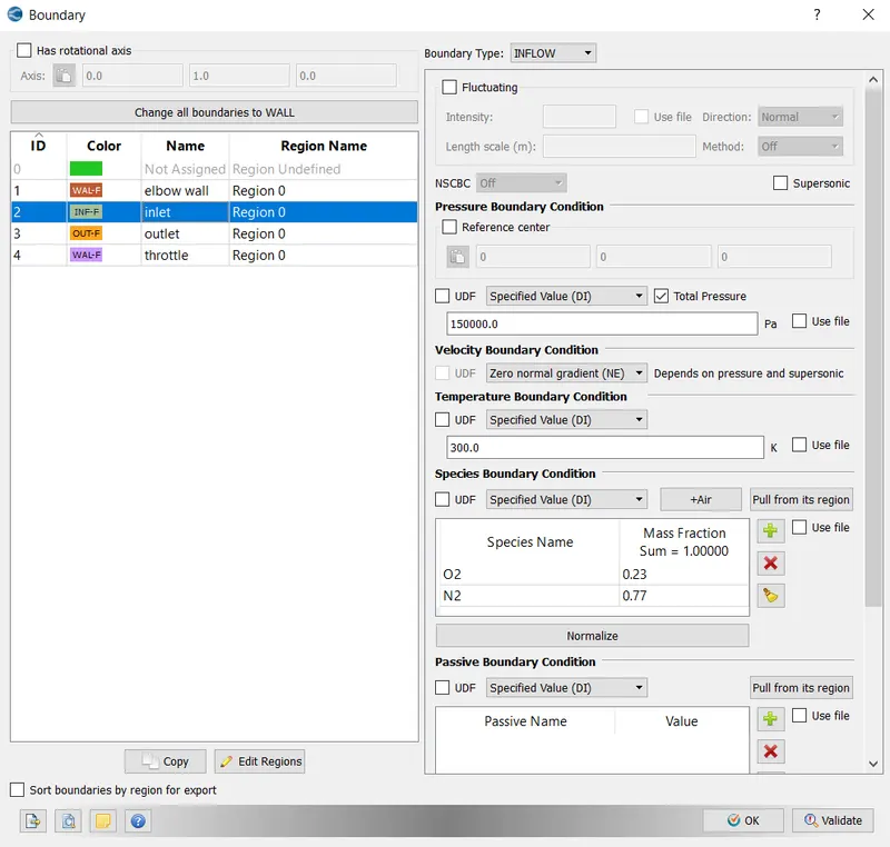
35. For inlet > > choose inflow type
36. 
37. 
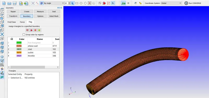
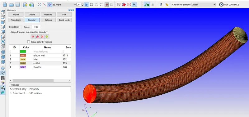
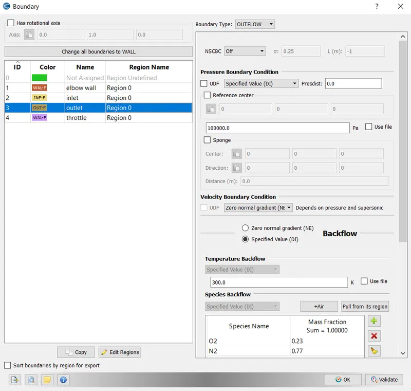
38. For outlet > > choose outflow type
39. 
40. 
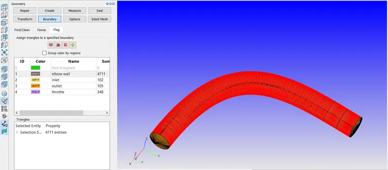
41. For elbow wall > > choose wall type
42. 
43. 
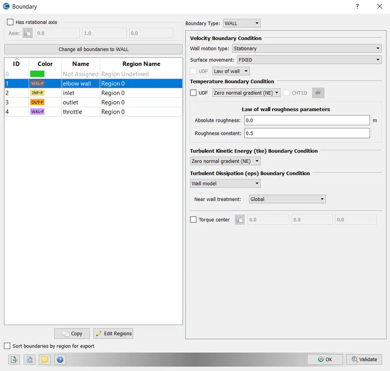
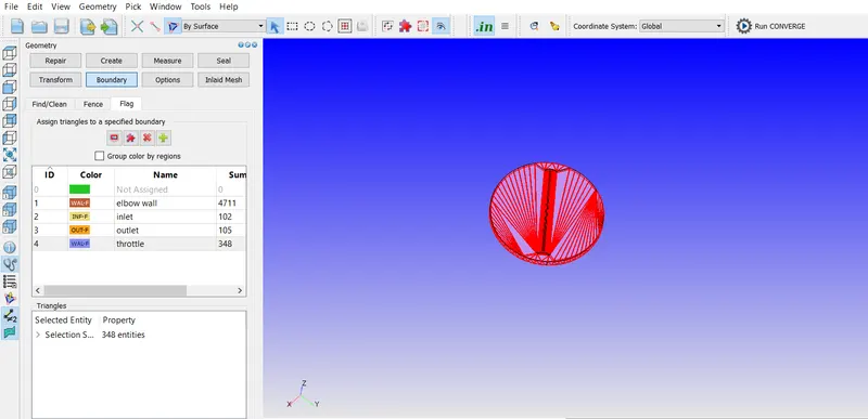
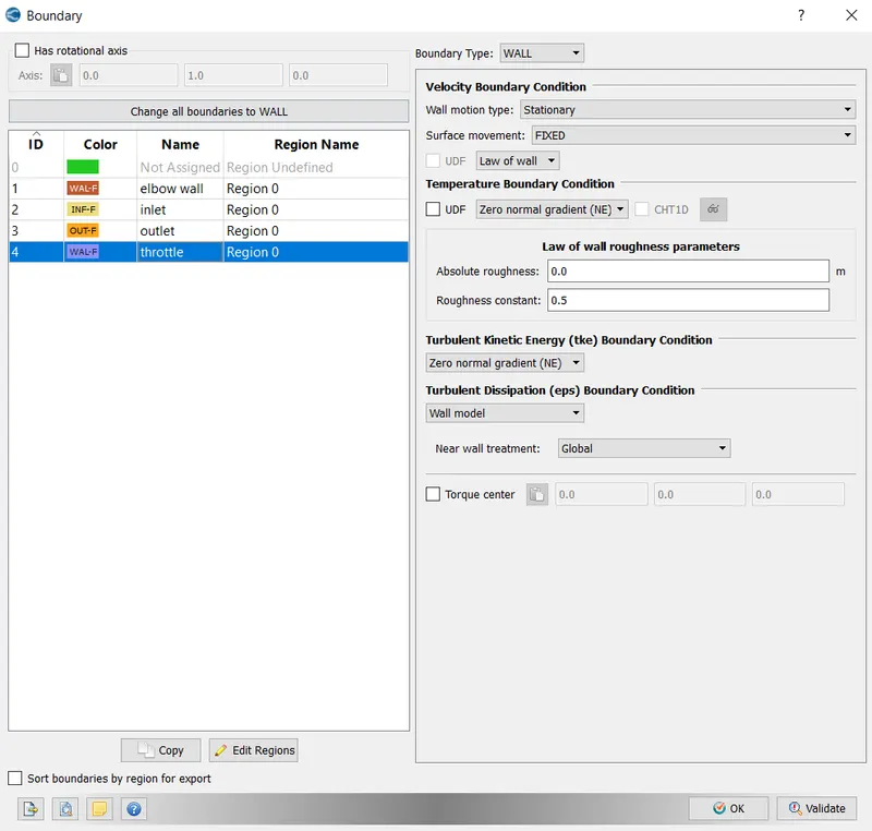
44. For throttle > > choose boundary type as wall
45. 
46. 
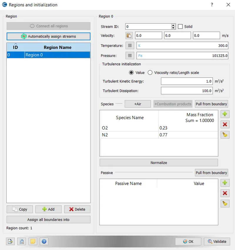
47. Go to initialization>> choose region give name as region0>> specify the composition of species
48. 
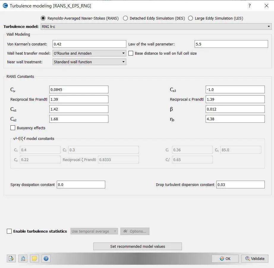
49. Go to turbulent model>> select RNG kepsilon
50. 
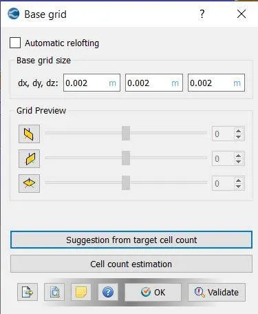
51. For grid control>> provide the grid sizes in x, y, z direction as 2mm
52. 
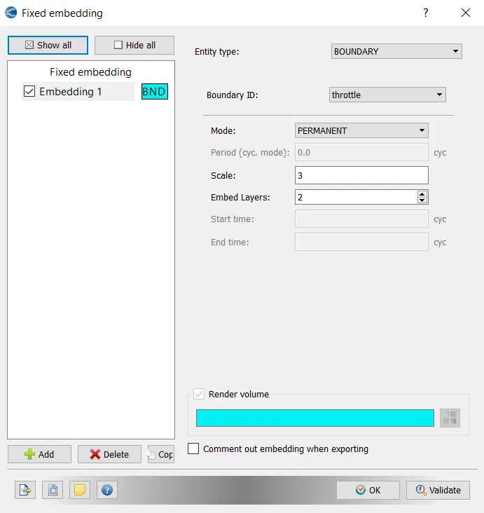
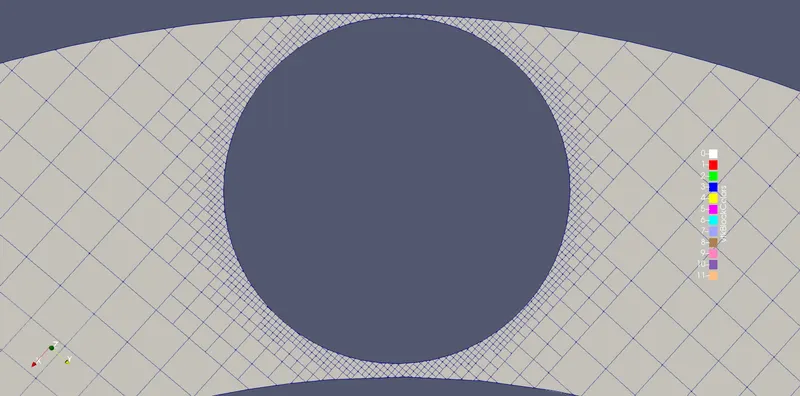
53. define fixed embedding to refine the grid at the throttle section>>select fixed embedding>>select boundary ID as throttle>>give embedding scale of 3 and layers 2
54. 
55. Go to post variable selection>> select the variables for post processing
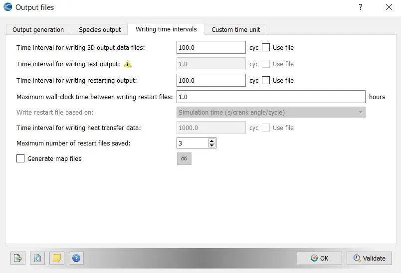
56. Go to output files>> provide the no of output files to be dumped.
57. 

Simulation run:

1. Export all the case set up from the converge studio
2. Go to Cygwin>> go to desired path or directory
3. Type the command mpiexec.exe -n 2 converge-intelmpi.exe to run the simulation.
4. To post convert the output files, go to Cygwin>> type the command as ex -n 2 post_convert_msmpi_64.exe

Post processing:

Meshing of the elbow wall region

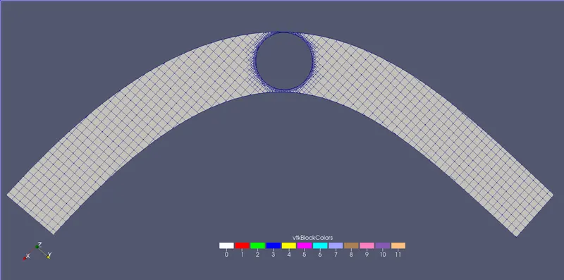
Meshing at the throttle section with embedding effect

Mass flow rate:

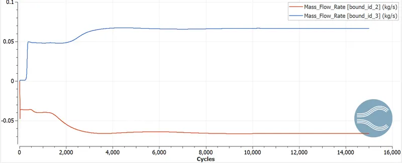
The mass flow rate is high initially and becomes stable at 0.007kg/s after reaching 10000 cycles. The fluctuation of mass flow is due to variation of inlet static pressure and decrease in velocity. The outlet mass flow rate increases and becomes stable at

Density variation:

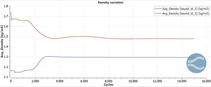
Inlet density variation is caused due to mass flow variation. The inlet density attains stability at 1.45kg/m3 after reaching 10000 cycles. At outlet section density increases and reaches stability at 1.3kg/m3 at 8000 cycles. The fluctuation is caused due to variation of mass flow at the throttle region.

Total pressure:

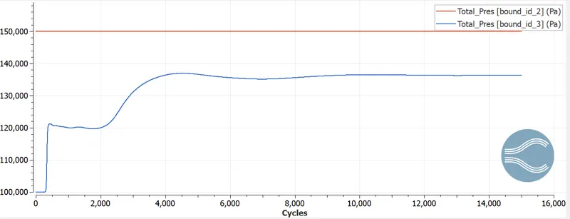
The inlet total pressure remains constant all over the cycles of iterations. The outlet pressure increases and becomes stable at 135000Pa after reaching 10000 cycles. This variation of pressure is due to mass flow moving at the outlet section from the corners of throttle wall and causing rise in total pressure.

Static pressure:

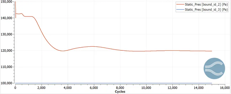
The inlet static pressure is very high initially and after encountering the valve gradually decreases and becomes stable at 12000Pa after reaching 10000 cycles. The outlet pressure remains constant because of less variation of mass flow at outlet.

Average velocity:

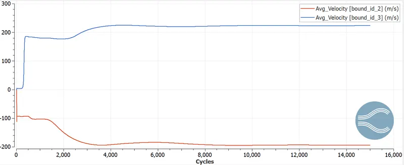
The inlet average velocity variation is very high at starting and then reaches stability at 190m/s after reaching 12000 cycles. The high outlet velocity is due to low is due to low static pressure difference at the throttle region.

Procesors used for computation:

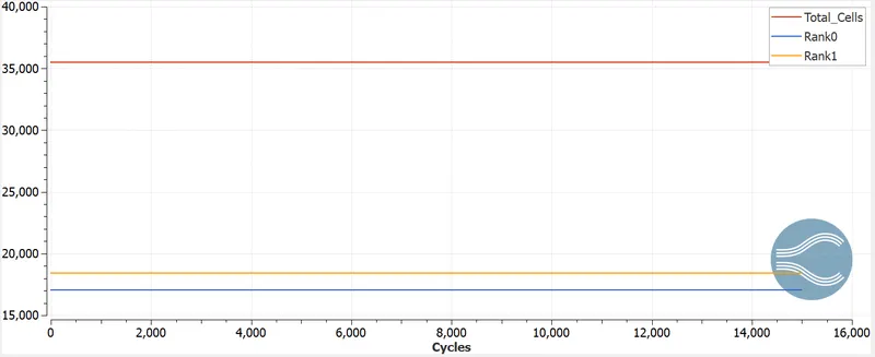
The total no of cell count used for running the simulation is around 36000 cells, while in processor 0 no of cells used is 17000 and for processor 1 no of cell count is 18500. the simulation is runned parallely in two processor to reduce the computational time.

Velocity:

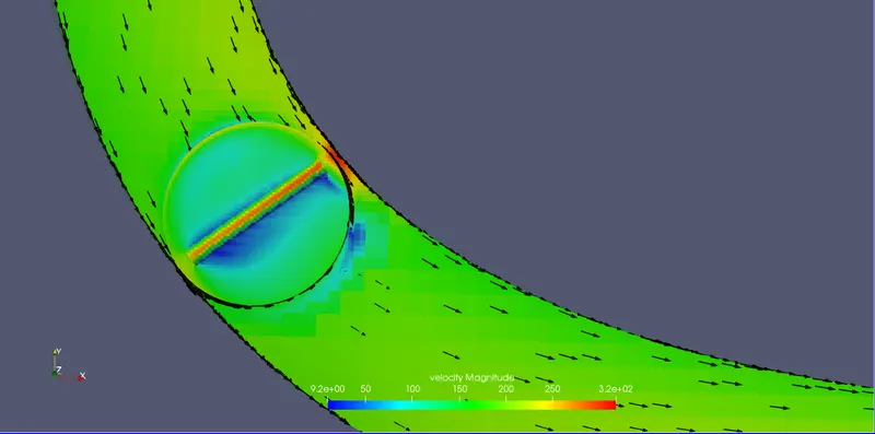
The velocity vector and the plane of throttle exposes the maximum velocity of 3.2e2m/s at the inlet section. While at the outlet section the velocity drops to 100m/s. The static pressure increases and the flow becomes seperated. the outlet velocity is low which supports low mass flow rate at the outlet.

Pressure:

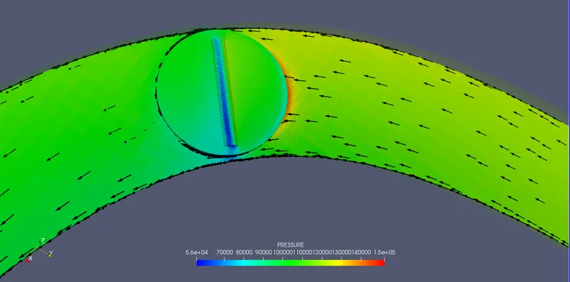
The inlet pressure is high and encountered at the throttlle front region and the magnitude is about 1.5e5Pa. The air while passing through the corners reduces the total pressure and flow seperation takes place. The pressure reaches around 80000Pa across the throttle corner sectiona and back portion.

Velocity animation:

Pressure animation:

Discussion:

From the steady state simulation of throttle valve, it is seen that pressure at the inlet is higher than the outlet. The mass flow variation is encountered at the throttle valve front position. The velocity at the inlet position is higher, but some region of high velocity is seen to leak from the corner of the throttle section. At the outlet the flow seeration takes place from the throttle surface and the outlet velocity reeduces down to attain a steady state value . The density variation also a function of mass flow variation and pressure difference. The flow seperation can be seen to take place when pressure tends to drop down.

Conclusions:

1. The steady state simulation is performed to observe the effect of flow seperation across the region of throttle section. The maximum velocity of 3.2e2m/s is observed at the inlet and low velocity of 50m/s at the outlet.
2. The pressure variation is seen to be fluctuating at the inlet and while encountering the valve, the pressure rises up. The outlet pressure becomes low and further detaches the flow seperation.
3. The grid refinement is done at the throttle section to capture accurately the flow behaviour. With refinement the computational cell count is higher and time taken to complete the simulation increases.