Flow over a backward facing step using CONVERGE CFD
Abstract:
In this project a backward face stepping geometry flow study is conducted. With different mesh sizes, the simulation is performed to observe output parameters like pressure, mass flow, velocity etc. The simulation set up is done in converge studio, run in Cygwin and post processed in ParaView.
Aim:
To analyse flow over a backward facing step at different grid sizes and observe the velocity and pressure distribution at the entire flow region.
Objective:
Run the case for three different base mesh sizes
- dx = dy = dz =2e-3m
- dx = dy = dz =1.5e-3m
- dx = dy = dz =1.0e-3m
1. Show the mesh (i.e surface with edges) for all the 3 base mesh sizes
2.Show pressure and velocity contours
3. Show the plots of velocity, pressure, mass flow rate and total cell count for all the 3 base mesh sizes
4. Also explain where and why separation is taking place in detail.
Introduction:
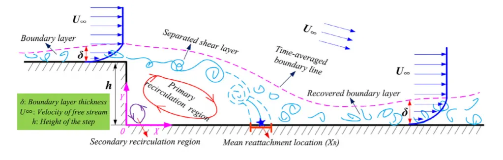
The backward facing step is an interesting case for studying the performance and solution strategy of a turbulence model. In this case, the flow is subjected to a sudden increase of cross-sectional area, resulting in a separation of flow starting at the point of expansion. Spatial variations in the velocity field cause production of turbulence outside the wall region and its interaction with the mean flow influences the size of the separation bubble. The size of the bubble, or the re-attachment length, is one of the quantities that must be predicted accurately by a turbulence model. Separation and reattachment of turbulent flows occur in many practical engineeringapplications, both in internal flow systems such as combustors and channelswith sudden expansions, and in external flows like those around airfoils and buildings.In these situations, the flow experiences an adverse pressure gradient, i.e. the pressureincreases in the direction of the flow, which causes the boundary layer to separatefrom the solid surface. The flow subsequently reattaches downstream forming arecirculation bubble. Among the flow geometries used for the studies of separatedlows, the most frequently selected is the backward-facing step. Considerable workhas been carried out on this flow due to its geometrical simplicity.
Backward-Facing Step (BFS) flow is one representative model for separation flows, which can be widely seen in aerodynamic flows (airfoil, spoiler, high attack angle process), engine flows, condensers, vehicles (cars, boat), heat transfer systems, and even the flow around buildings, etc. The flow separation after a simple stage will introduce separation bubble formation, evolution and re-attachment process, which is dependent on the BFS geometric design, the inlet and outlet conditions, turbulent intensity, as well as heat transfer conditions. In the past decades, it has been widely studied by various theoretical, experimental and numerical methods. Considering the importance of BFS flow in both theoretical and engineering aspects, this paper is focused on a review study of BFS flows from fundamental understandings to various experimental and numerical developments in a historical viewpoint. Basic models and the parameter-based after-step flow laws are summarized and categorized in this study. It is shown that the step size (duct expansion ratio) will define the basic re-circulation and re-attachment process, while the coupled effects of inflow parameters.
Basic features and theoretical aspect of Backward-Facing Step
The Backward-Facing Step (BFS) flows, also called as “sudden expansion flows”, “circular expanding flow”, “back-step flow”, “diverging channel” or “backward flow” under some other occasions, involves the basic features of general separation flows. It has three-dimensional nature and suitable for two-dimensional discussions under some flow conditions and/or with simple step geometry. It is an important model for separation flows across wide range of Reynolds numbers. This section describes the features and major theoretical challenges in BFS flows.The flow field of BFS is also generally divided into four regions: separated shear layer, the recirculation region under the shear layer, the reattachment region, and the attached/recovery region.From theviewpoint of a flow dynamics, the BFS flow happens with large separation vortices in the backward step region and with some small vortex in the corner. Sometimes complex vortex series will also happen under different Re and geometric conditions. Between the separation bubble and the mainstream flow a free shear layer can be found, slight different from that of a plane shear layer due to the existence of separation bubble. The shear layer then develops and finally form re-attachment on downstream boundary.
Case setup:
- Open converge studio console
- Drop and drag the created geometry.
- from option tab create bounding box.
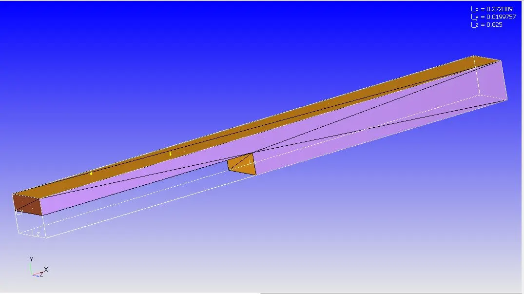
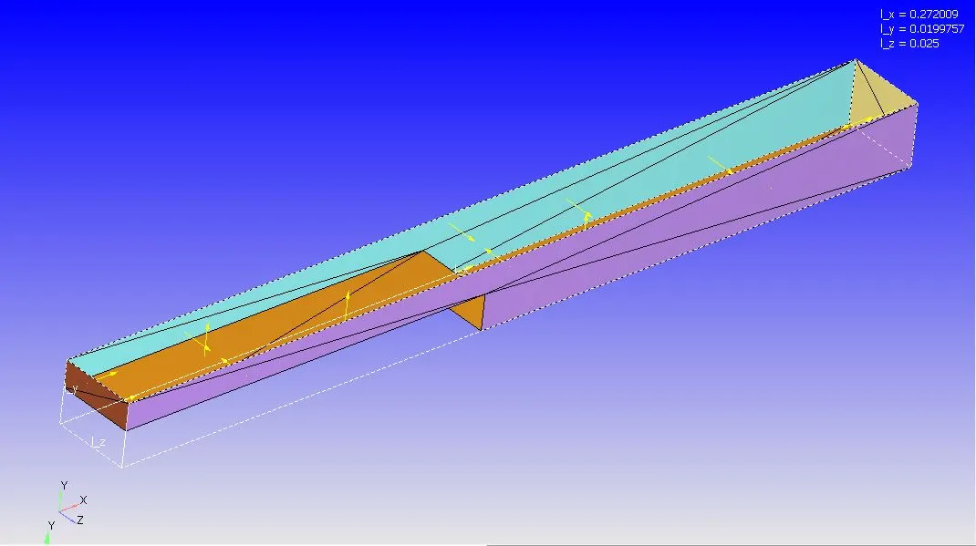
- The normal vectors of geometry are pointed inside.
- Go to the right-hand side case set up option, there we will find many setting up option.
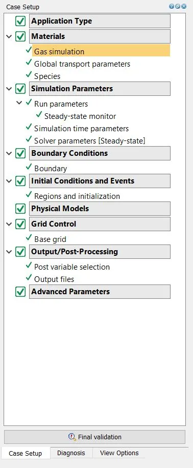
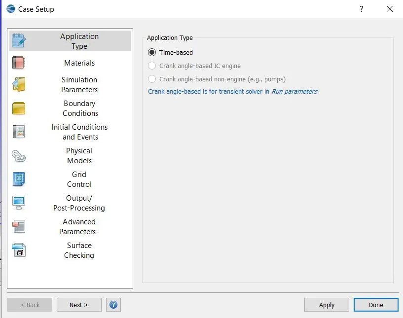
- Select application option>>select time based option.
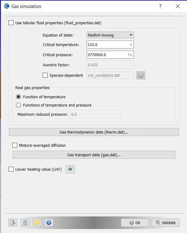
- Go to materials>> select gas simulation >> click ok
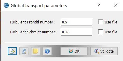
- Go to global transport parameters >> select ok.
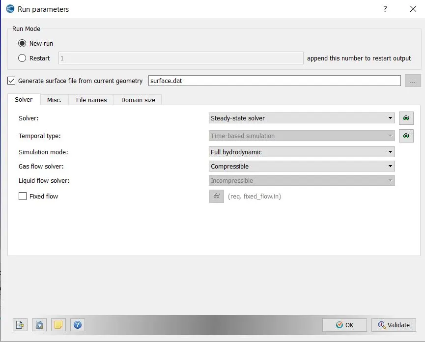
- Go to simulation parameters>> select run parameters>> choose steady state solver with full hydrodynamic case.
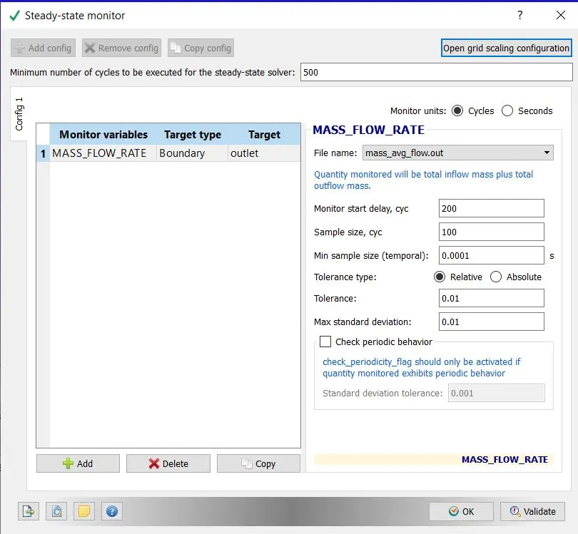
- Go to steady state monitor>> provide monitor variable as mass flow rate>> select target type boundary>> select target as outlet
- Provide the min no of cycles for steady state solver>> provide monitor delay start, sample size.
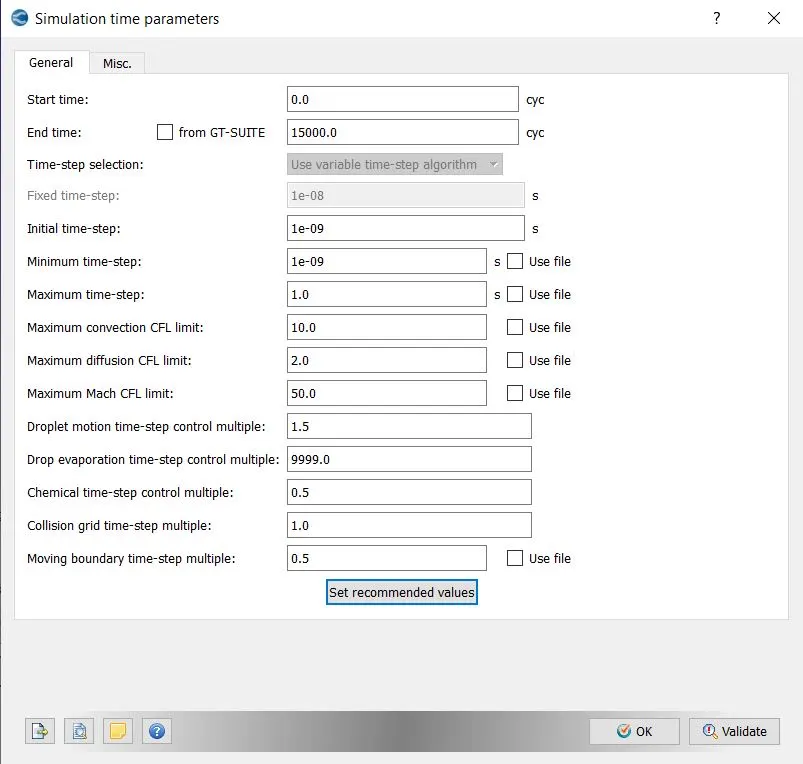
- Select simulation time parameter>>provide end time as 15000 cycles>> provide initial and min time step of 1e-6 and max time step of 1
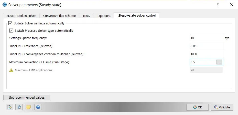
- Go to solver parameter setting>> choose density based >> go to equation >>select pressure and set precondition to none>> go to solver control and define the cfl limit to 0.5
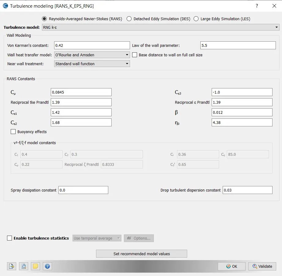
- choose turbulent model as kepsilon.
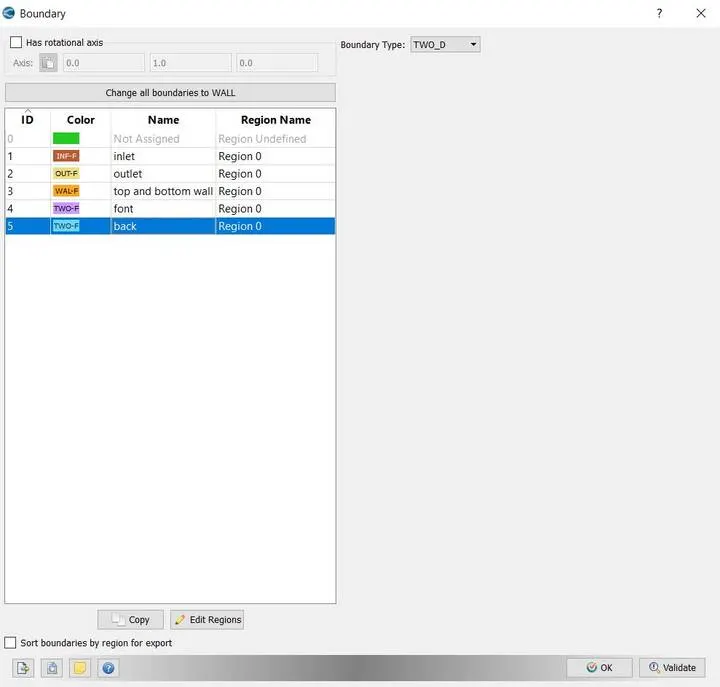
- Go to boundary>> define all boundary region name with ID
- For inlet > > choose inflow type
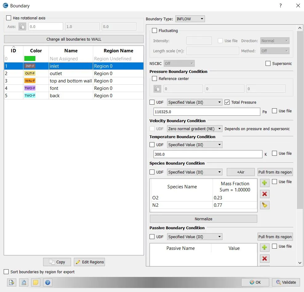
- For outlet > > choose outflow type
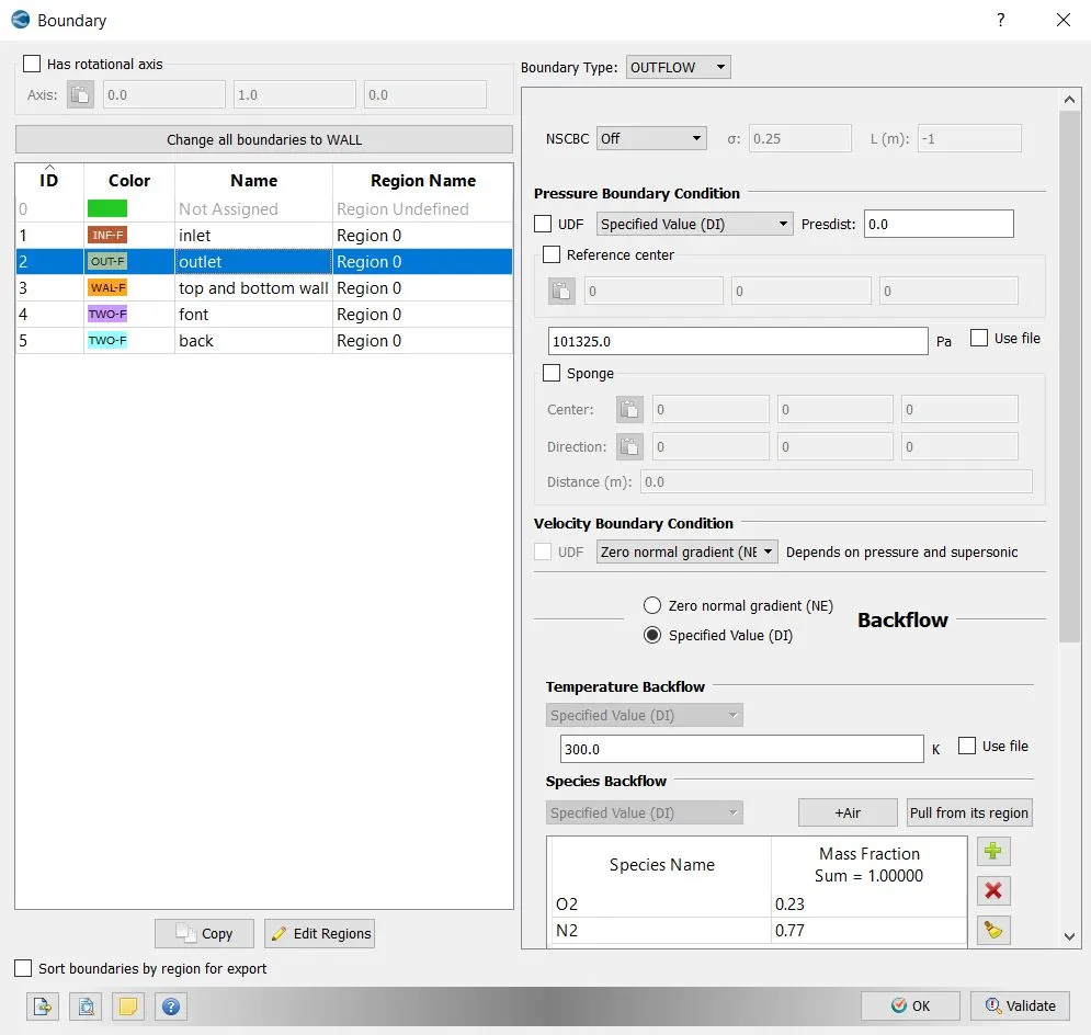
- For top and bottom > > choose wall type
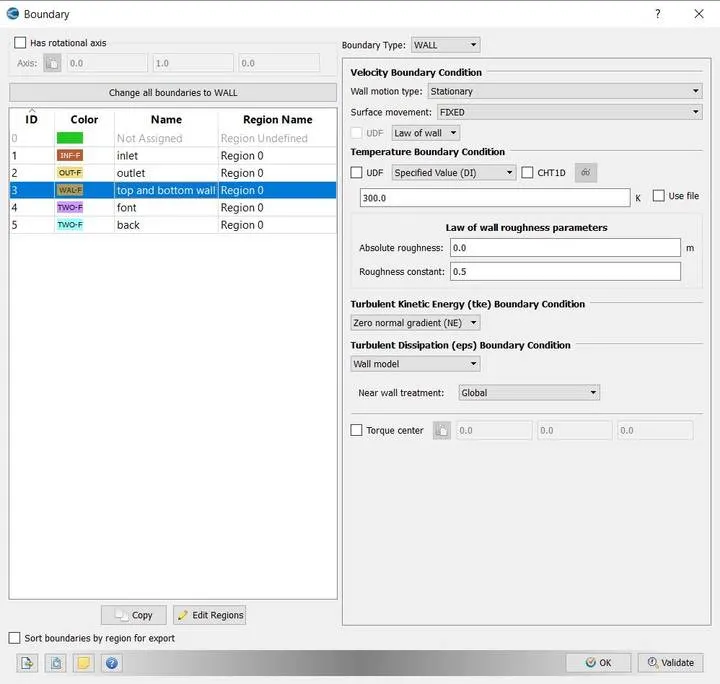
- For front and back > > choose 2D type
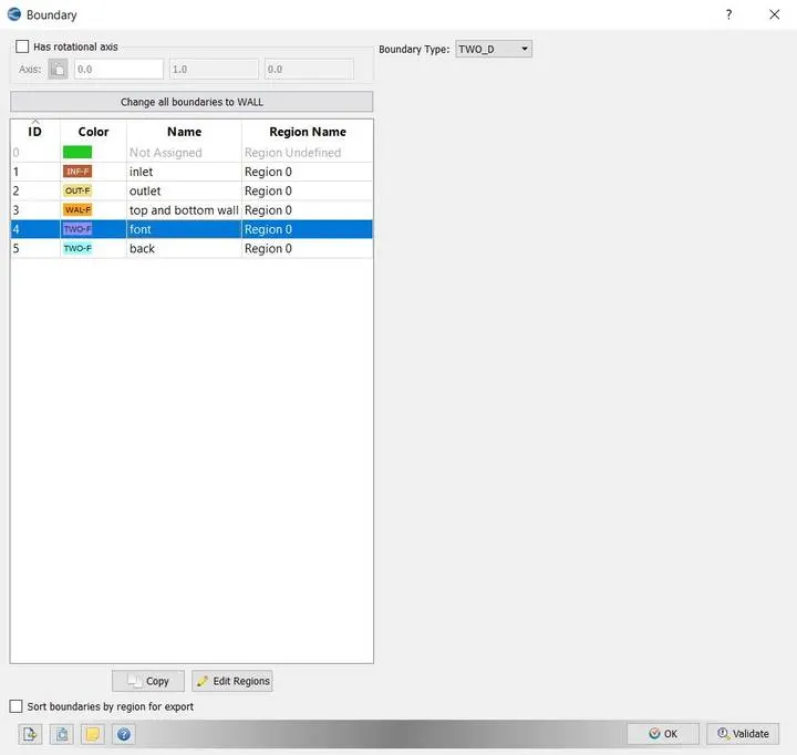
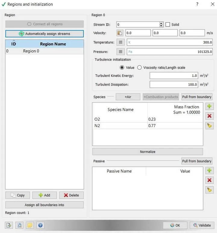
- Go to initialization>> choose region give name as volumetric region>> specify the composition of species
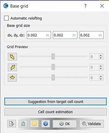
- For grid control>> provide the grid sizes in x, y, z direction as per different cases
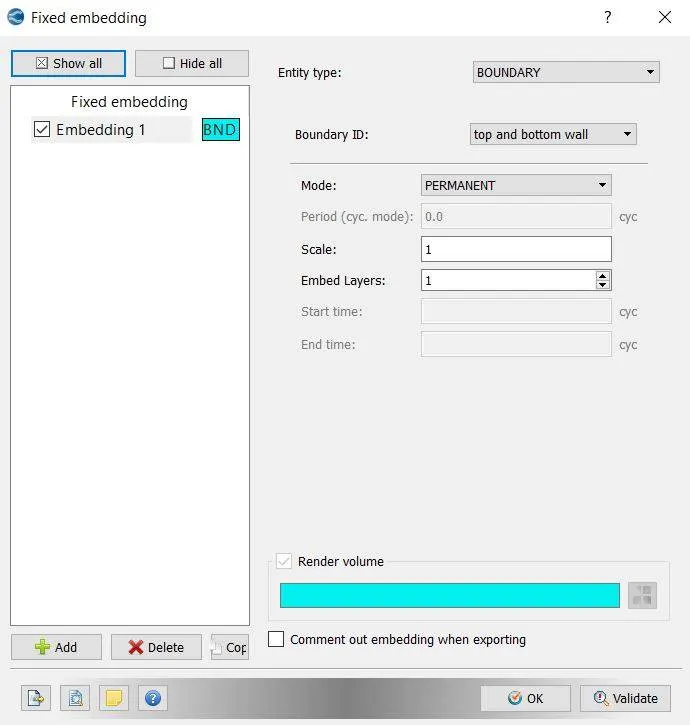
- Define fixed embedding for refining the grid at the boundary regions>> select fixed embedding>> select boundary ID as top and bottom wall>> provide scale factor of 1.
- Go to post variable selection>> select the variables for post processing
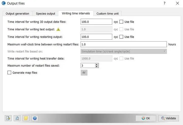
- Go to output files>> provide the no of output files to be dumped.
Simulation run:
- Export all the case set up from the converge studio
- Go to Cygwin>> go to desired path or directory
- Type the command mpiexec.exe -n 2 converge-intelmpi.exe to run the simulation.
- To post convert the output files, go to Cygwin>> type the command as ex -n 2 post_convert_msmpi_64.exe
Case setup:
Different mesh size cases and post processing plots and animation:
- Mesh size: 2e-3
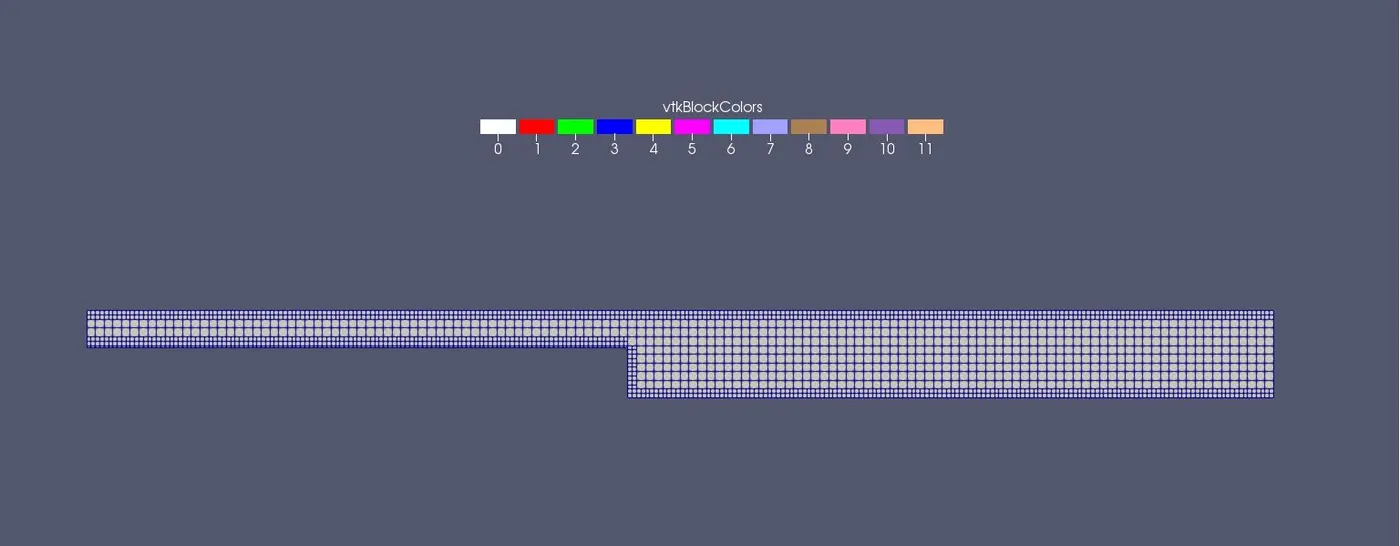
Mesh geometry
Mass flow rate:
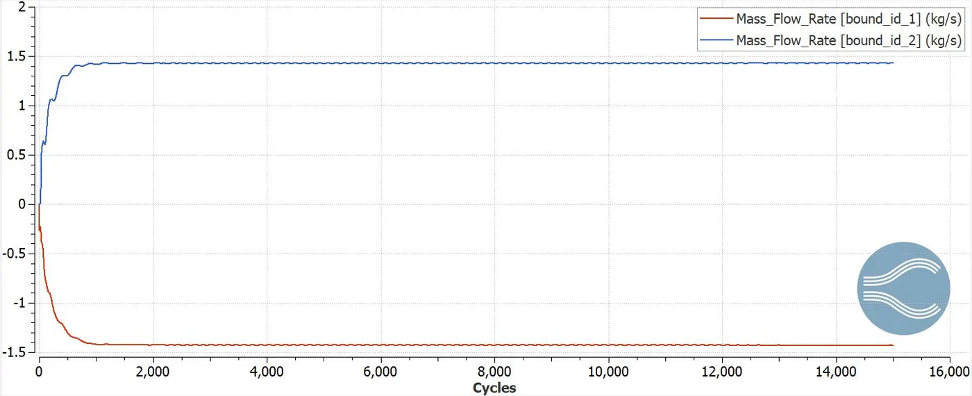
The initial mass flow rate is very high and becomes stable at 1.4kg/s after reaching 2000 cycles. The outlet mass flow also attains stability at 1.4 kg/s after reaching 2000 cycles. This fluctuation of mass flow rate is because of increase in pressure difference and decrease in velocity at the outlet.
Total pressure:
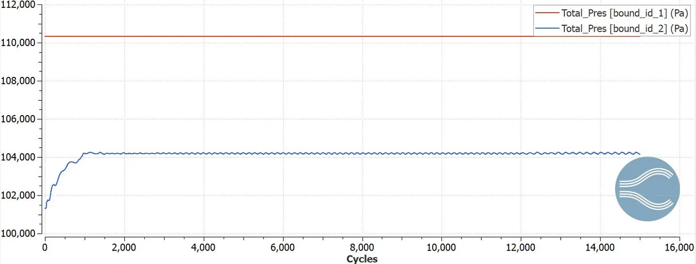
The inlet total pressure is constant at 101325Pa for all cycles and outlet pressure reaches a stable value of 104000Pa for 2000 cycles. The average velocity becomes a factor of decrement due to increase in magnitude.
Static pressure:
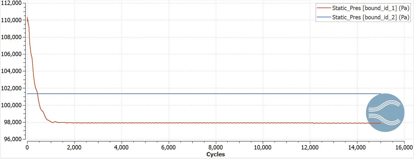
The inlet static pressure becomes stable at 98000Pa after reaching 2000 cycles. The outlet static pressure remains constant over all the cycles of operation because of outlet velocity.
Average velocity:
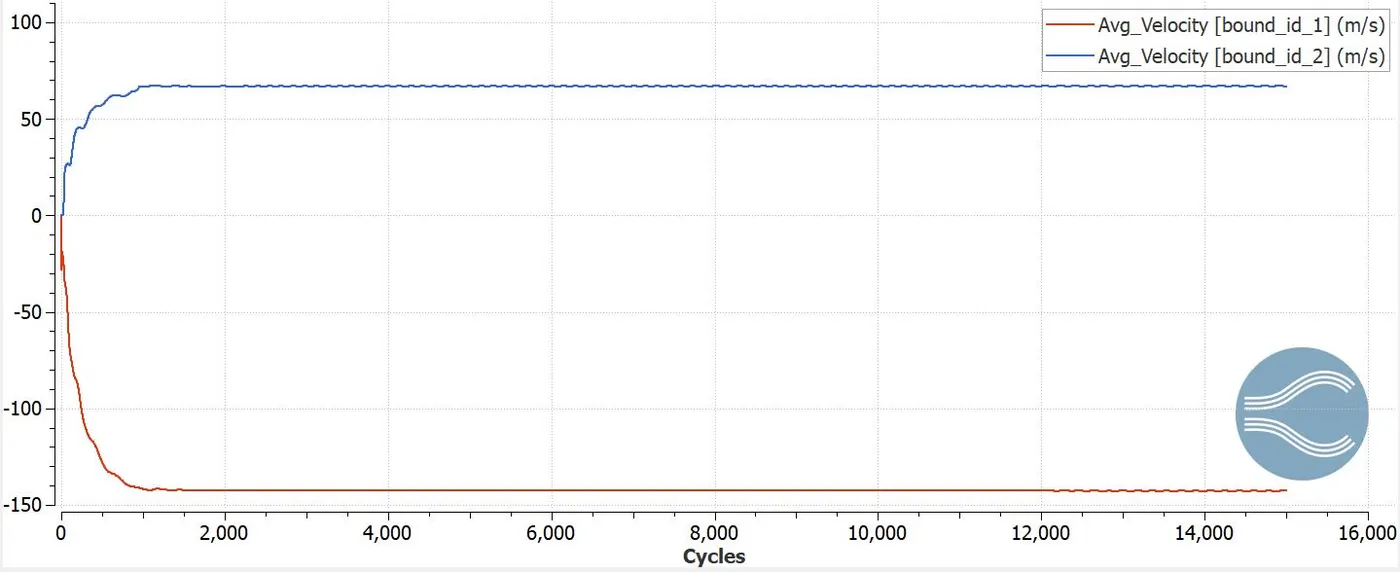
The avg inlet velocity is very high and becomes stable at 139m/s after reaching 2000 cycles. The outlet velocity reaches stability at 69m/s after reaching 2000 cycles. The velocity stability depends upon mass flow rate, it is exactly at the same cycle reached by mass flow rate to attain the stable value.
Total cell count:
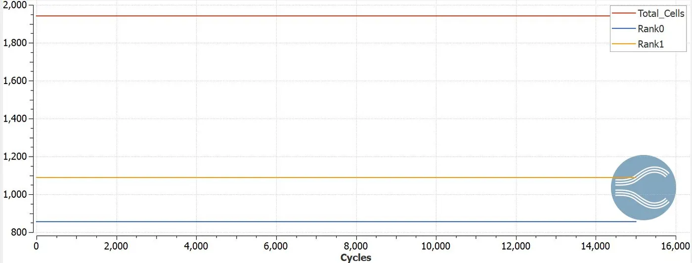
The total cell count stands to 1900 cells, and for processor 1 it counts 800 cells and for processor 2 it counts 1100 cells.
Velocity magnitude:
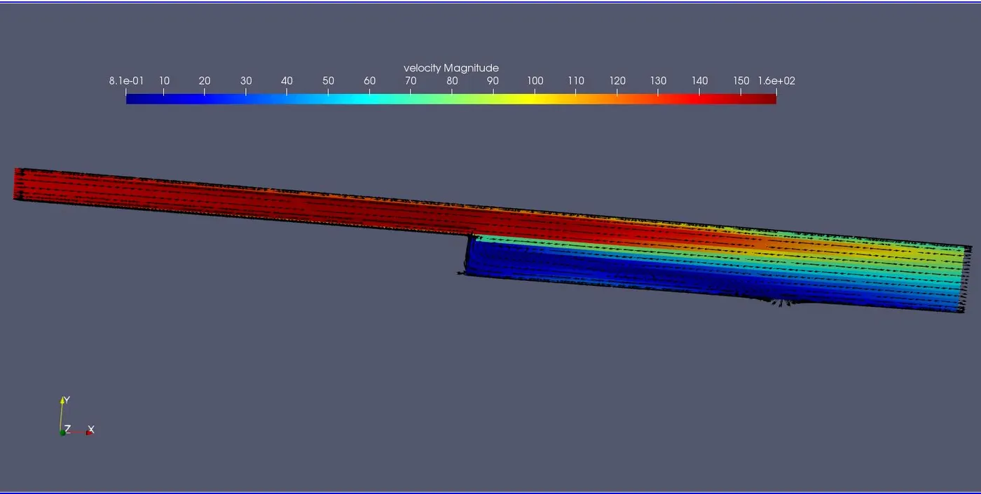
As seen from the vector plots the air circulation tends to recirculate around the stepped region. The max velocity of 160m/s and minimum velocity of 81m/s is achieved which indicates the decrease in pressure at the outlet.
Pressure magnitude:
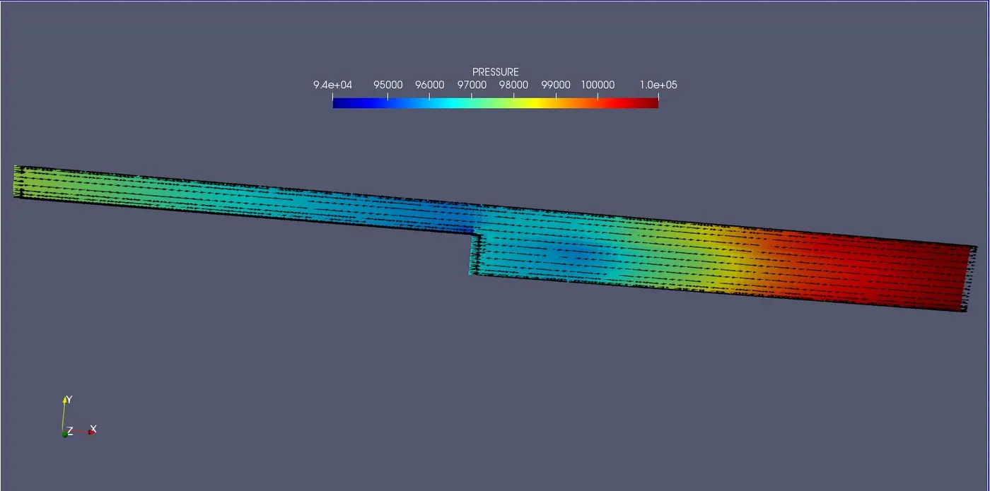
The pressure magnitude goes from lower to higher as air moves from inlet to outlet section. The max pressure of 1e5 and min pressure oof 9.4e4 is achieved. The zone of high pressure is seen at the outlet which necessarily predicts low velocity at outlet.
Post processing animation:
Velocity contour:
Pressure contour:
- Mesh size: 1.5e-3
Mesh geometry
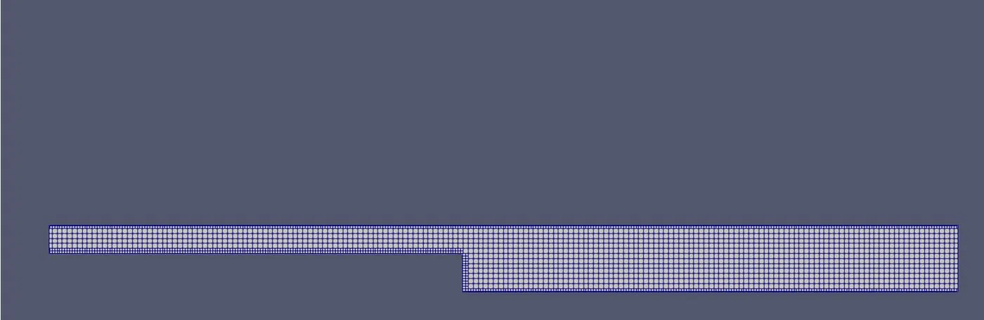
Inlet mass flow rate:
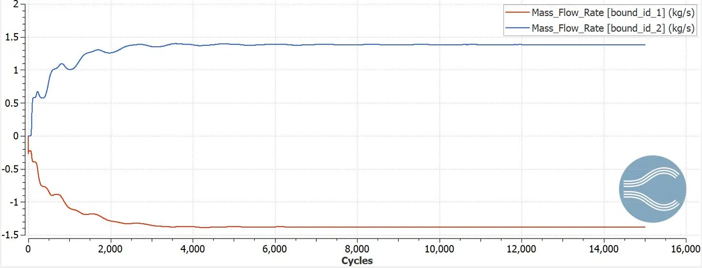
The initial mass flow rate is very high and becomes stable at 1.3kg/s after reaching 6500 cycles. The outlet mass flow also attains stability at 1.3 kg/s after reaching 6500 cycles. This fluctuation of mass flow rate is because of increase in pressure difference and decrease in velocity at the outlet.
Total pressure:
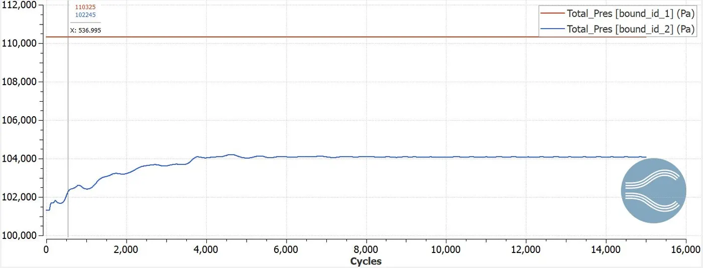
The inlet total pressure is constant at 101325Pa for all cycles and outlet pressure reaches a stable value of 104000Pa for 10000 cycles. The average velocity becomes a factor of decrement due to increase in magnitude.
Static pressure:
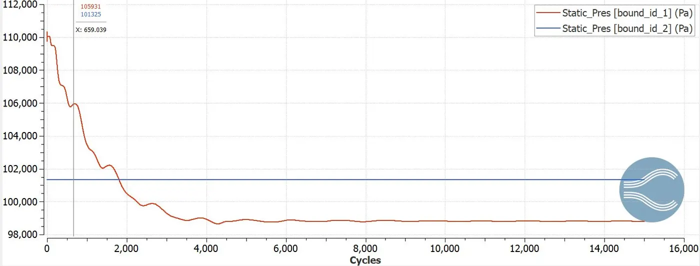
The inlet static pressure becomes stable at 98000Pa after reaching 10000 cycles. The outlet static pressure remains constant over all the cycles.
Average velocity:
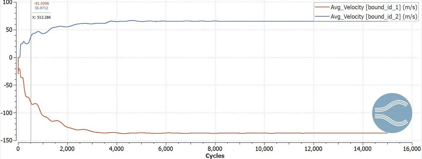
The avg inlet velocity is very high and becomes stable at 130m/s after reaching 12000 cycles. The outlet velocity reaches stability at 65m/s after reaching 8000 cycles. The velocity stability depends upon mass flow rate, it is exactly at the same cycle reached by mass flow rate to attain the stable value.
Total cell count:
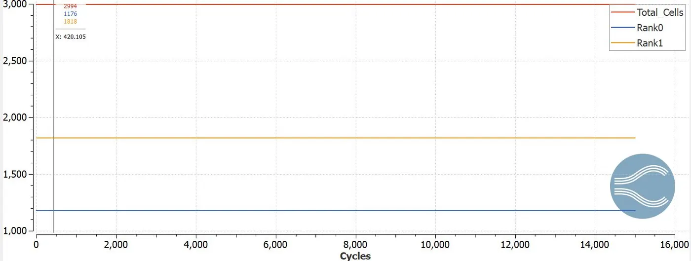
The total cell count stands to 3000 cells, and for processor 1 it counts 1100 cells and for processor 2 it counts 1800 cells.
Velocity magnitude:
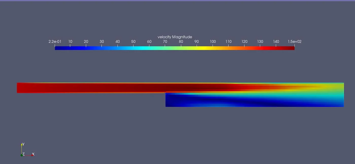
As seen from the vector plots the air circulation tends to recirculate around the stepped region. The max velocity of 150m/s and minimum velocity of 0.2m/s is achieved which indicates the decrease in pressure at the outlet.
Pressure magnitude:
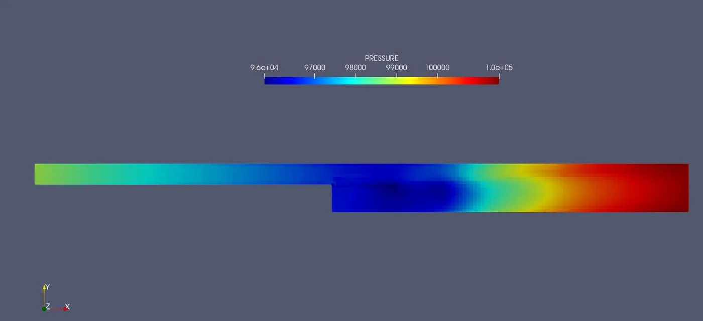
The pressure magnitude goes from lower to higher as air moves from inlet to outlet section. The max pressure of 1e5 and min pressure oof 9.4e4 is achieved. The zone of high pressure is seen at the outlet which necessarily predicts low velocity at outlet.
Post processing animation:
Velocity contour:
Pressure contour:
- Mesh size: 1e-3
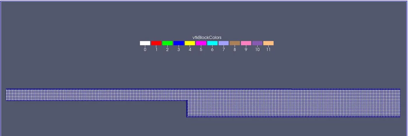
Mesh geometry
mass flow rate:
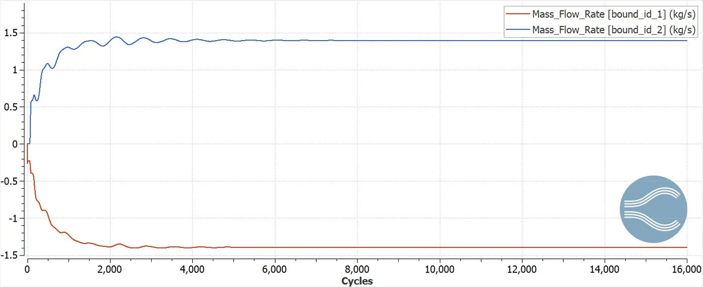
The initial mass flow rate is very high and becomes stable at 1.4kg/s after reaching 5000 cycles. The outlet mass flow also attains stability at 1.4kg/s after reaching 8000 cycles. This fluctuation of mass flow rate is because of increase in pressure difference and decrease in velocity at the outlet.
Total pressure:
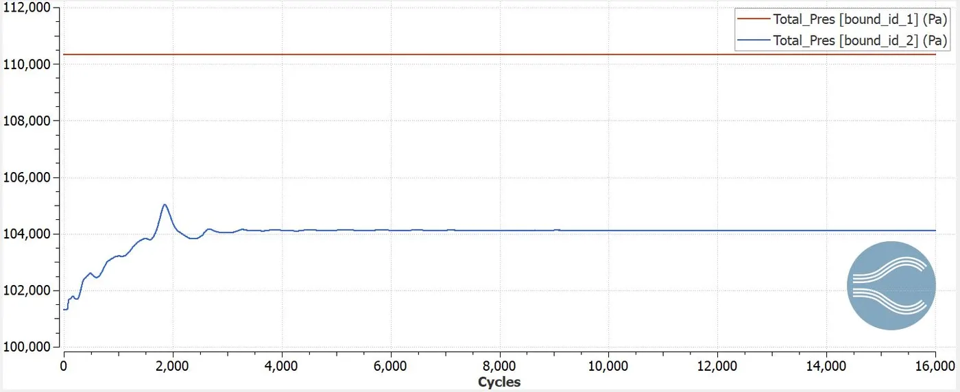
The inlet total pressure is constant at 101325Pa for all cycles and outlet pressure reaches a stable value of 104000Pa for 10000 cycles. The average velocity becomes a factor of decrement due to increase in magnitude.
Static pressure:
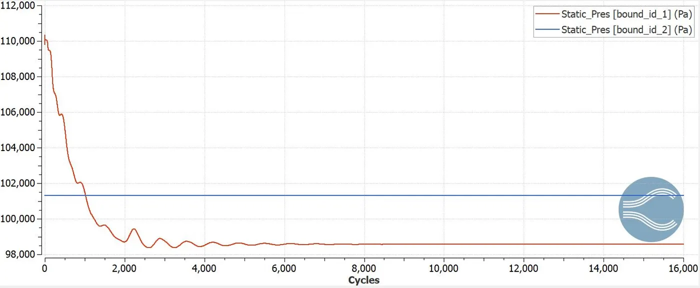
The inlet static pressure becomes stable at 98000Pa after reaching 9000 cycles. The outlet static pressure remains constant over all the cycles.
Average velocity:
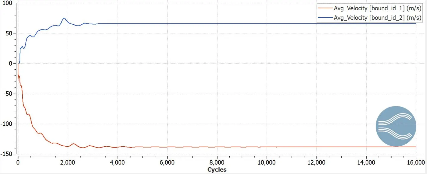
The avg inlet velocity is very high and becomes stable at 140m/s after reaching 5000 cycles. The outlet velocity reaches stability at 60m/s after reaching 4000 cycles. The velocity stability depends upon mass flow rate, it is exactly at the same cycle reached by mass flow rate to attain the stable value.
Total cell count:
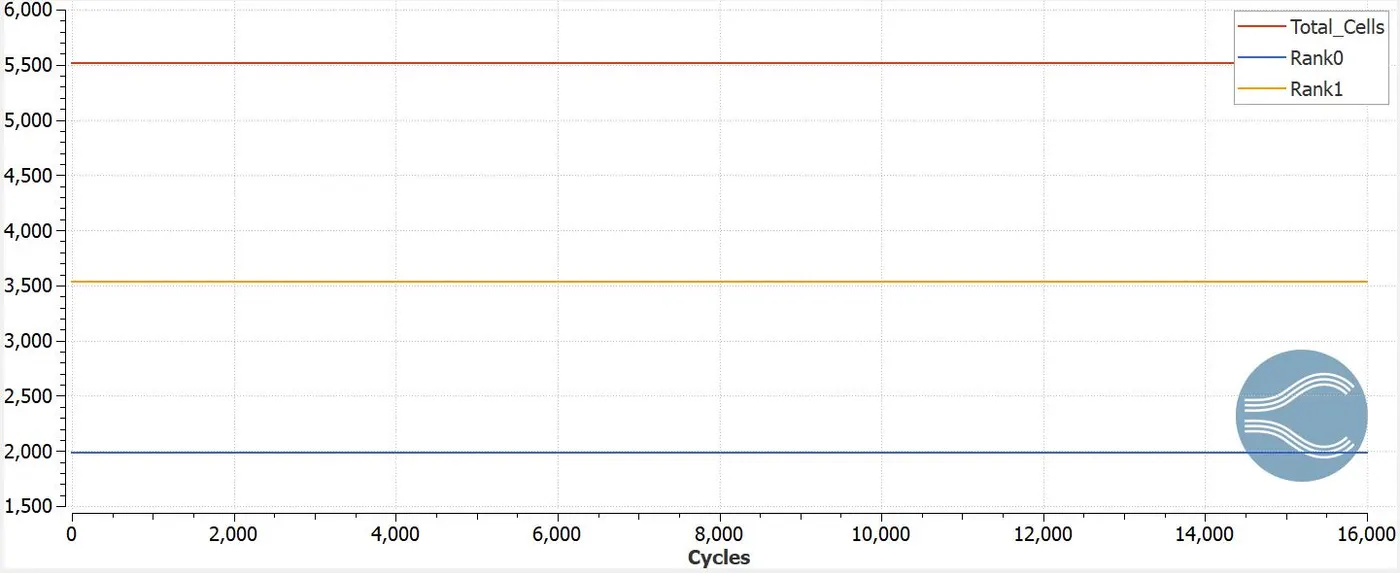
The total cell count stands to 1900 cells, and for processor 1 it counts 800 cells and for processor 2 it counts 1100 cells.
Velocity magnitude:
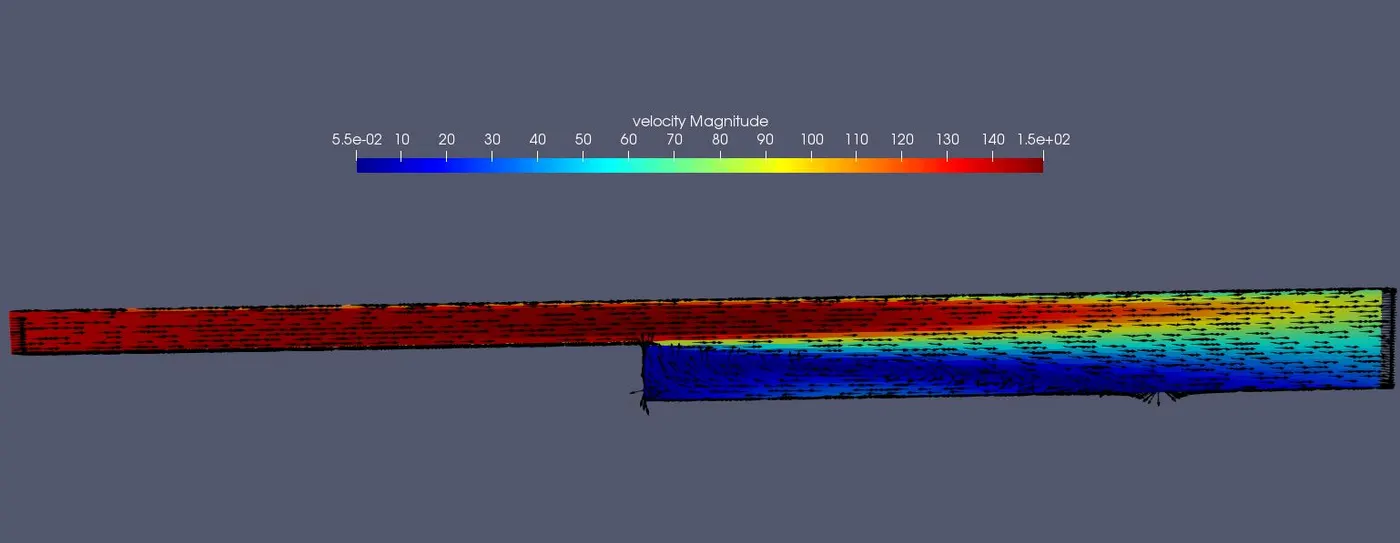
As seen from the vector plots the air circulation tends to recirculate around the stepped region. The max velocity of 150m/s and minimum velocity of 0.05m/s is achieved which indicates the decrease in pressure at the outlet.
Pressure magnitude:
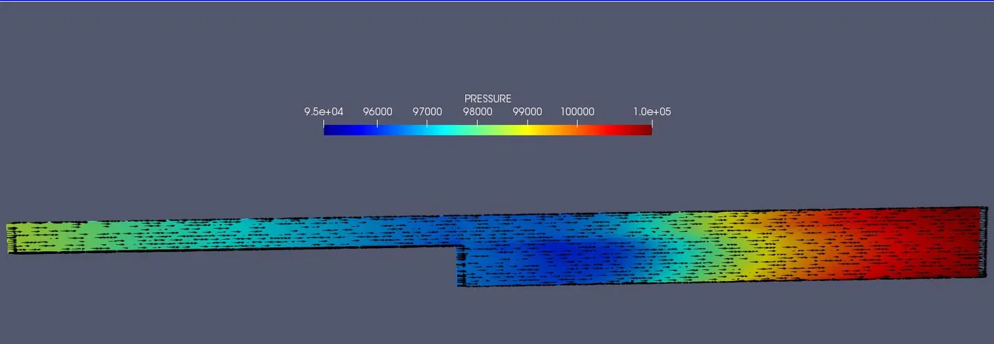
The pressure magnitude goes from lower to higher as air moves from inlet to outlet section. The max pressure of 1e5 and min pressure oof 9.4e4 is achieved. The zone of high pressure is seen at the outlet which necessarily predicts low velocity at outlet.
Post processing animation:
Velocity contour:
Pressure contour:
Discussions:
It is seen that mass flow rate becomes stable at 1.4kg/s for the 3 cases, only difference is that with more refinement the no of cycles to attain the stability increases. From the outlet velocity point of view, the magnitude of velocity decreases with increase in mesh sizes. This is also due to increase in static pressure generated at the outlet section for various cycle of iterations. The velocity vector and pressure magnitude direction also informs about the separation formation taking place due to boundary layer effect and recirculation of pressure zone where velocity reduces and pressure increases at the cost of it.
Seperation of flow analysis for different mesh sizes:
The inlet velocity is maximum, however it drops suddenly at the flow separation region where the cross section of the geometry increases and the region of recirculation gets created. The vector plots of velocity shows the necessary circulation captured during the process. Pressure drop is maximum at the outlet, but at the cross section it reduces suddenly. This recirculation pattern creates turbulent formation of flow. After then the velocity and the pressure gains stability and steadily moves towards the outlet section. The inlet and the outlet mass flow rate has also converged to satisfy the conservation principle. For the first mesh size the velocity at the recirculating zone is 60m/s, for the second mesh size it is 30m/s and for the third case it is 10m/s. This proves that on refining the mesh, the boundary layer can be captured more effectively. With quality embedding at the region, the flow separation can be observed in more details.
Conclusions:
- With increase in mesh size, the total no of cell counts increases, which increases the computational time and cost of simulation.
- with increase in mesh quality, the boundary layer capture can be done in a more refined way and the no of cycles required to achieve stability for diffrerent parameters increases.
- the flow field velocity and pressure recirculation zone can be captured with more refining the order of mesh. thw magnitude of max velocity fairly matches with the graphical data plots.