Week 6.2 - Setting up a model (Hanging Node)

Problem statement

1. The Icepak model is given for this assignment. Open and unpack the given hanging_node.tzr model.

Without any modifications, the model results in about 700,000 elements. Note that this mesh count results from using the non-conformal meshing technique, which reduces mesh bleeding and mesh count. However, this mesh does not fully resolve the fine-level geometric features of the CAD objects. You can reduce the mesh count and improve the mesh resolution on and around the CAD objects by using the multi-level meshing technique. This procedure starts with a coarse background mesh and resolves fine level features through a series of successive mesh refinements. By using multi-level meshing and the uniform mesh parameters feature, you can reduce the mesh count to approximately 500,000 elements and improve mesh resolution.

2. Generate the Mesh:
   1. Create non-conformal mesh assembly
   2. Use mesh separately option with slack values
   3. Use object parameters
   4. Use set uniform parameters and use average on 1 assembly, in multi-level meshing tab allow multi-level meshing up to level 2 for the objects.
   5. Use the same technique of 1
   6. Generate mesh.
   7. Observe in mesh reduction
   8. Do visual inspection
   9. Check for quality
3. solve the model using the flow condition. Consider forced convection based analysis.

Model

File>> open>> unpack model>> hangingnode.tzr file- this opens the model and click on view>> default shading- solid

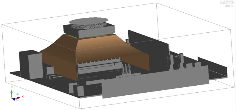
This model has two CAD models

Sheet metal HS

Fan guide sweep

The mesh refinement is done to capture the model accurately. The mesh modelling is done using coarse method to reduce the mesh count and mesh bleeding by non-conformal technique.

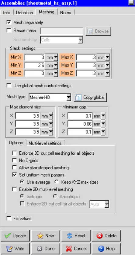
Sheet metal Assembly settings:

Slack settings for assembly meshing

Min x = 3mm

Max x =3mm

Min y= 2.6 mm

Max y= 3 mm

Min z = 3mm

Max z = 3mm

Mesh type

Maximum element size in x = 3.5 mm

Maximum element size in y = 3.5 mm

Maximum element size in z = 3.5 mm

Min gap x = 0.1mm

Min gap y = 0.06mm

Min gap z = 0.1mm

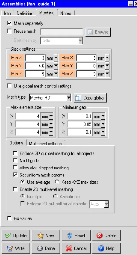
Fan guide Assembly settings:

Slack settings for assembly meshing

Min x = 3mm

Max x =3mm

Min y= 0

Max y= 4.6 mm

Min z = 3mm

Max z = 9mm

Mesh type

Maximum element size in x = 4mm

Maximum element size in y = 4mm

Maximum element size in z = 4mm

Min gap x = 0.1mm

Min gap y = 0.05mm

Min gap z = 0.1mm

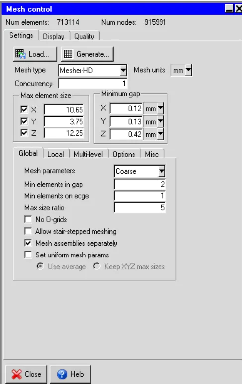
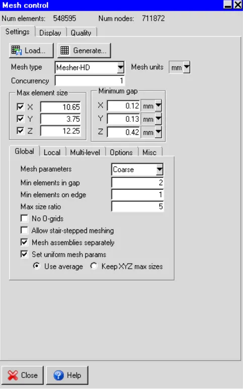
Global mesh settings:

Maximum element size in x = 10mm

Maximum element size in y = 3.75mm

Maximum element size in z = 12.5mm

Min gap x = 0.12mm

Min gap y = 0.13mm

Min gap z = 0.42mm

Mesh parameter: coarse

Visual inspection

final mesh count

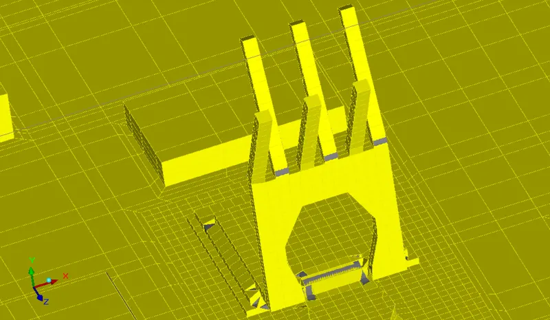
Sheet metal

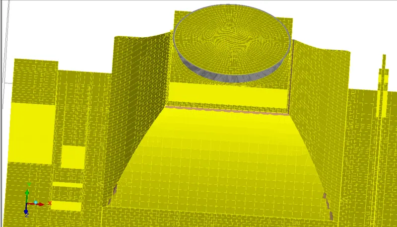
Fan guide

Meshing along x direction

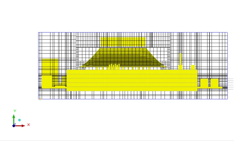
Meshing along y direction

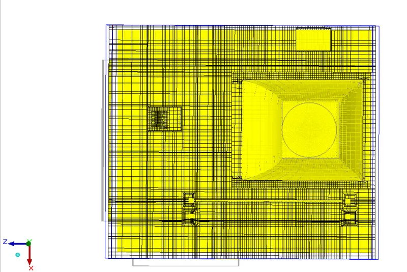
Meshing along z direction

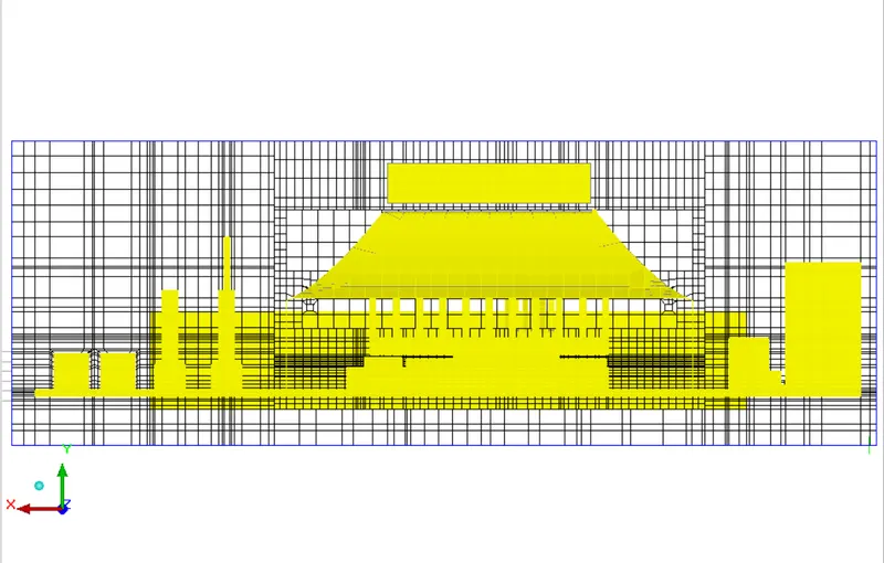
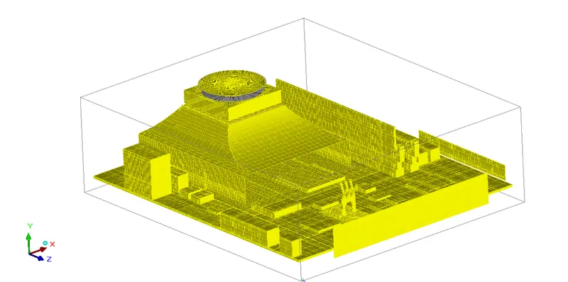
Overall mesh

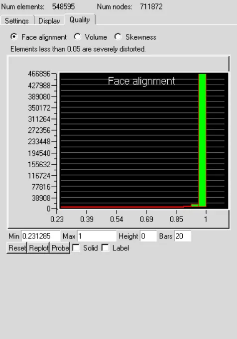
Mesh verification:

Face alignment:

Measures the mesh quality by face alignment index.

The value of face alignment ranges from 0 to 1. Value greater than 0.1 is preferred and greater than 0.15 is better.

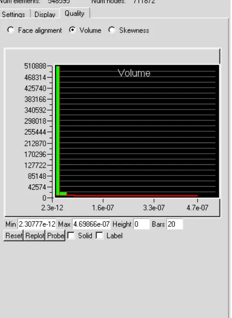
Volume:

Preferable volume mesh should be 1e-12 for single precision and 1e-15 for double precision.

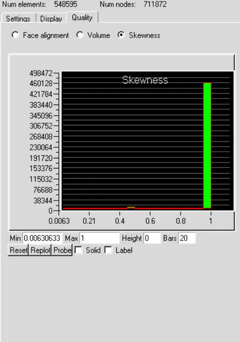
Skewness:

It determines the deviation of the mesh from its ideal shape.

Physics setup:

Solver: 3D navier stokes solver is used to study the computational domain.

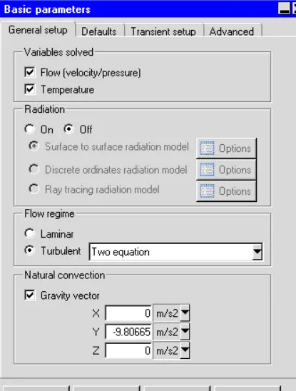
General set up:

Boundary conditions

basic parameters

Turbulent model: two equation

Radiation: off

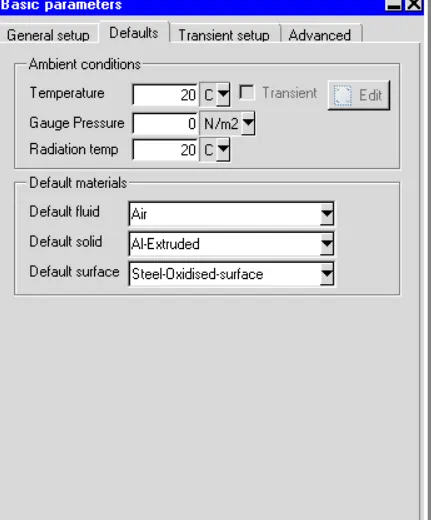
Flow conditions

Temp 20 degree

Pressure 0Pa

Radiation temp 20degree

Default fluid air

Default solid extruded Al

Transient setup: steady

solution initialization

x velocity: 0

y velocity: 0

z velocity: 0

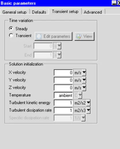
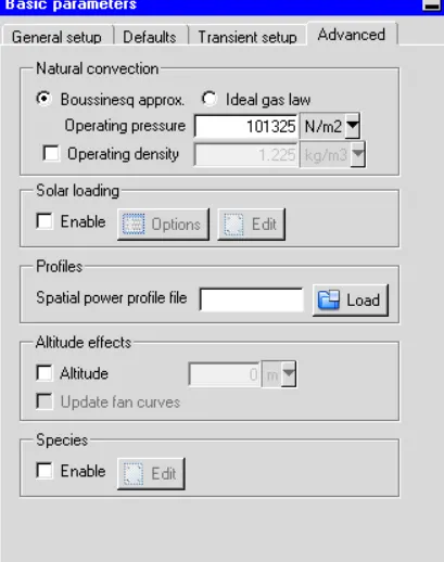
Natural convection bc

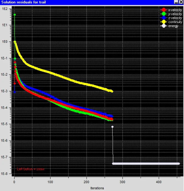
No of iterations: 1000

Flow convergence: 0.001

Energy convergence: 1e-10

Joule heating: 1e-7

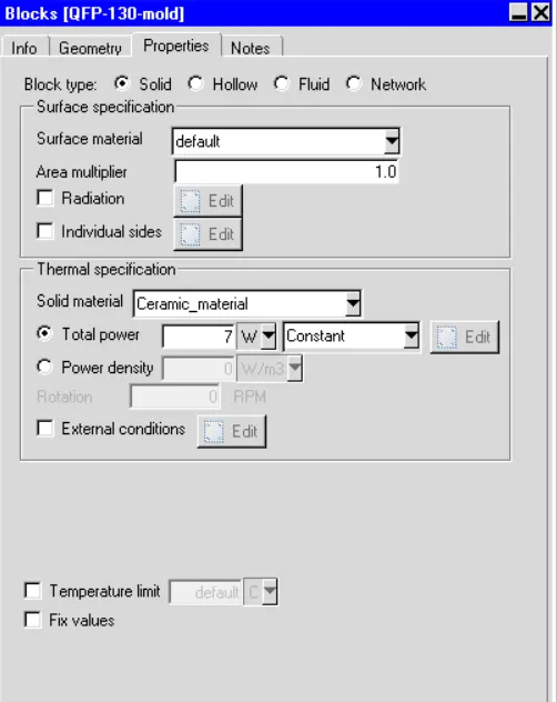
Sheet metal assembly BC

Material: ceramics

Power source: 7W

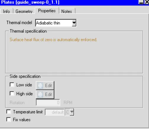
Fan BC

Fan guide sweep

Thermal model: adiabatic thin

Fan type: internal

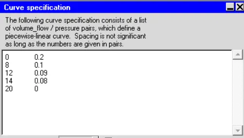
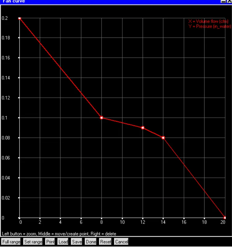
Flow type: non linear

Curve specification

Swirl rpm: 4000

Parallel setup: 2 processors

Post processing plots

Convergence plot

Monitor points:

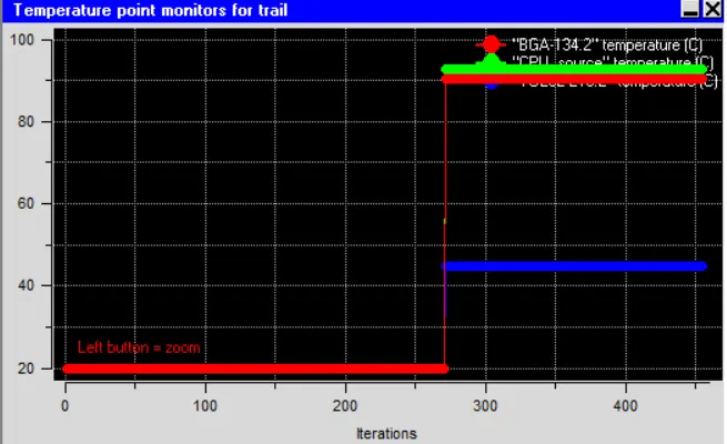
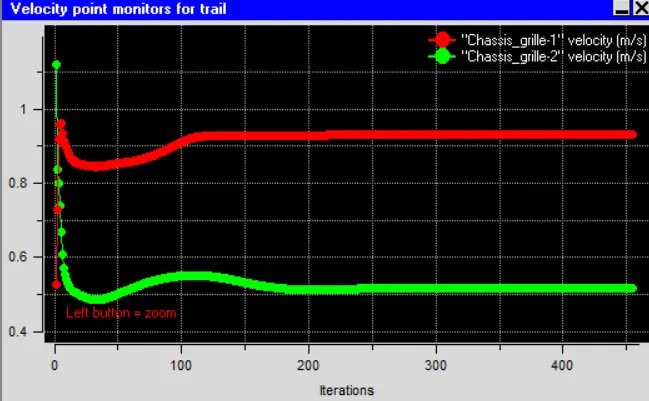
Temperature and velocity monitor points are set up at various key location within computational domain. Apart from providing information about solution variables, it also helps to determine the solutions steady state condition.

Temperature monitor:

The temperature monitor plot shows temperature values on three objects are given below

BGA 134.2- 95.98degree

CPU source- 92.22degree

T0252- 44.45degree

Velocity monitor:

The velocity monitor points are defined on two objects of computational domain given as

Chassis grille 1- 0.931m/s

Chassis grille – 0.512m/s

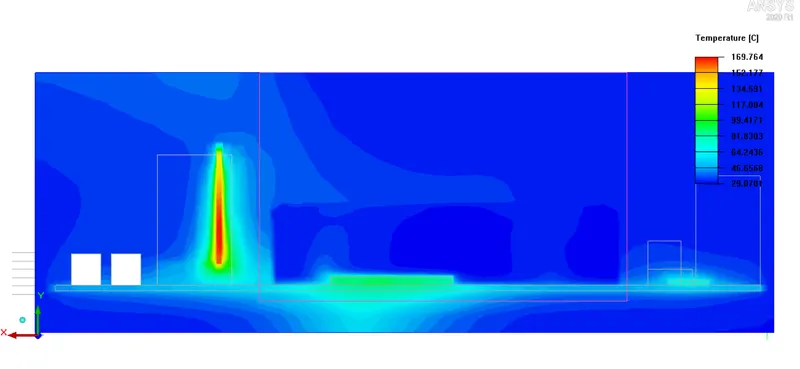
Temperature object contour

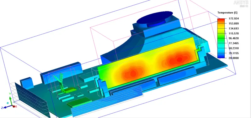
The contour shows that air in the assembly is at lower temperature compared to other objects. As a result, the air leaving the domain is hotter than entering it. The maximum temperature is found to be 172 degrees.

Temperature in X axis

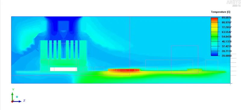
Temperature in Y axis

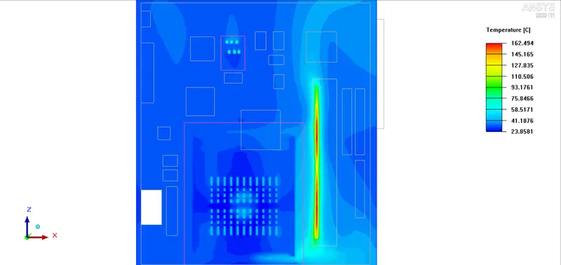
Temperature in Z axis

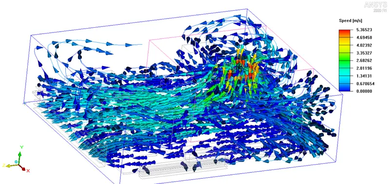
Velocity vector plot

Velocity vector plot in X axis

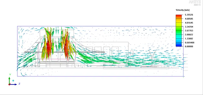
Velocity vector plot in Y axis

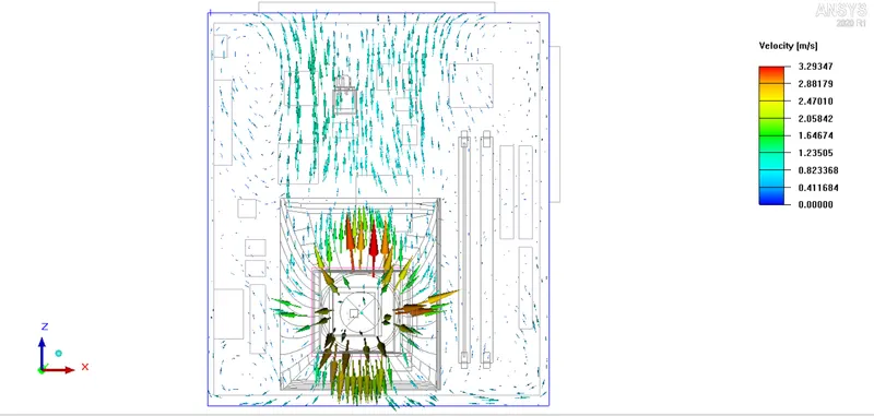
Velocity vector plot in Z axis

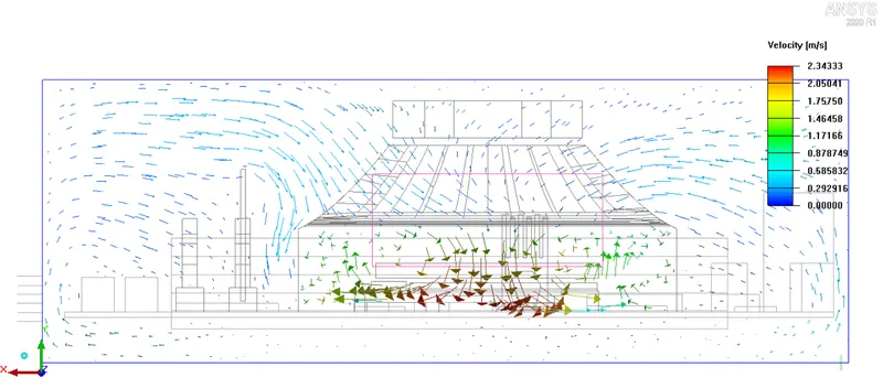
Velocity in X axis

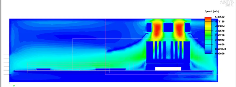
Velocity in Y axis

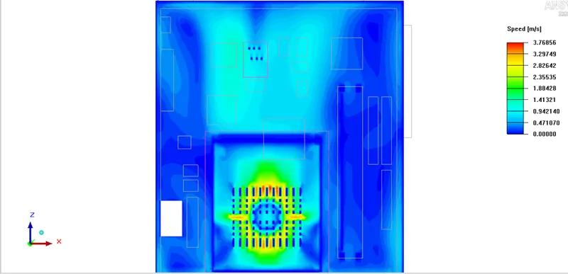
Velocity in Z axis

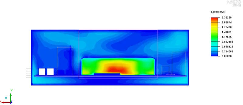
Conclusions:

• Multilevel meshing is performed on the sheet metal and fan guide assembly to reduce the mesh bleeding and mesh cell count appreciably to get accurate results.
• The temperature contour has spotted a maximum temperature of 172 degrees in the domain, which is effectively cooled by the circulating air, thereby maintaining the thermal conditions.
• The velocity contour and vector plots indicate the direction of air flow inside the domain. Forced convection by the fan shows effective cooling by recirculating the air across the domain.