Numerical analysis of a Linear system of equation in MATLAB

Aim: To study the linear systems using iterative solver techniques.

Objective:

• to compute the eigen values of an iteration matrix
• compute spectral radius of the matrix
• solve the system using jacobi, gauss seidel and sor solver.

Governing equation:

The general form of linear system in matrix is

AX=B

Where A is coefficient matrix, B is the constant matrix and X are unknown variables to be determined.

In terms of iterative approach, we can solve the values of x by fixed point method

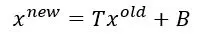
Where T is the iteration matrix.

The iteration matrix can be determined by different iterative solvers which are given below:

• Jacobi method

Here D, L, U represent the diagonal, lower and upper triangular matrix.

The iteration matrix is

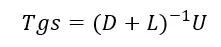
• Gauss Seidel method

The iteration matrix is

• Successive over relaxation method

The iteration matrix is

The spectral radius of the iteration matrix is given by

Given:

A=[5 1 2 ; -3 9 4; 1 2 -7]

X=[x1;x2;x3]

B=[10 -14 33]

Algorithm:

• define the range of magnification factor (0.5-2).
• three function call is provided for each value of magnification factor.
• Each function call returns the no of iteration, spectral radius, x_new and analytical spectral radius.
• Inside each function call the diagonal matrix is changed with magnification factor, the lower and upper triangular matrix are also defined.
• A convergence loop is defined where new values of x gets updated with each new iteration matrix. The error is computed with difference between old and new x values.
• At the main program the plot between no of iteration and spectral radius is plotted and magnification factor with no of iterations,magnification factor with spectral radius and comparison plot between computed and analytical spectral radius.

MATLAB code

main program code

clc
clear all
close all
%define the range of magnification factor
magnification_factor=linspace(0.5,2,100);
%define the coefficient matrix
A=[5,1,2;-3,9,4;1,2,-7];
%%%%%%%%%%%%% function declaration for linear system of equation%%%%%%%%%%%%%

for i=1:length(magnification_factor)
    m=magnification_factor(i);%stores each value of magnification factor
    %function call for jacobi solver
    [jac_iter(i),x_new,rho_j(i)]=jacobi_stability(m);
  %stores new values of x matrices
    x1_j(i)=x_new(1,1);
   x2_j(i)=x_new(2,1);
   x3_j(i)=x_new(3,1);
   %function call for gauss siedel solver
    [gs_iter(i),x_new_gs,rho_gs(i)]=gs_stability(m);
    %stores new values of x matrices
   x1_gs(i)=x_new_gs(1,1);
   x2_gs(i)=x_new_gs(2,1);
   x3_gs(i)=x_new_gs(3,1);
   %function call for SOR solver
     [sor_iter(i),x_new_sor,rho_sor(i)]=sor_stability(m);
     %stores new values of x matrices
   x1_sor(i)=x_new_sor(1,1);
   x2_sor(i)=x_new_sor(2,1);
   x3_sor(i)=x_new_sor(3,1);
    
end

%%%%%% function for calculating analytical spectral radius%%%%%%

for i=1:length(magnification_factor)
    m=magnification_factor(i);
    [rho_ana_j(i),rho_ana_gs(i),rho_ana_sor(i)]=analytical_spectral_radius(m);
    
end
%%%%%%%%%%%%%%%%%%%%%%%%%%%%%%%%%%%%%%%%%%%%%%%%%%%%%%%%%%%%%%%%%%%%%%%%

figure(1)
plot(magnification_factor,rho_j)
xlabel('diagonal dominance magnification factor')
ylabel('spectral radius of jacobi iterative solver')
titletext1=sprintf('diagonal dominance vs spectral radiusn');
titletext2=sprintf('JACOBI SOLVER');
title([titletext1 titletext2])
figure(2)
plot(magnification_factor,rho_gs)
xlabel('diagonal dominance magnification factor')
ylabel('spectral radius of gauss siedel iterative solver')
titletext1=sprintf('diagonal dominance vs spectral radiusn');
titletext2=sprintf('GAUSS SIEDEL SOLVER');
title([titletext1 titletext2])
figure(3)
plot(magnification_factor,rho_sor)
xlabel('diagonal dominance magnification factor')
ylabel('spectral radius of SOR iterative solver')
titletext1=sprintf('diagonal dominance vs spectral radiusn');
titletext2=sprintf('SUCCESSIVE OVER RELAXATION SOLVER');
title([titletext1 titletext2])
%%%%%%%%%%%%%%%%%%%%%%%%%%%%%%%%%%%%%%%%%%%%%%%%%%%%%%%%%%%%%%
figure(4)
plot(rho_j,jac_iter)
xlabel('spectral radius of jacobi iterative solver')
ylabel('no of iterations for jacobi solver')
titletext1=sprintf('no of iteration vs spectral radiusn');
titletext2=sprintf('JACOBI SOLVER');
title([titletext1 titletext2])
figure(5)
plot(rho_gs,gs_iter)
xlabel('spectral radius of gauss siedel iterative solver')
ylabel('no of iterations for gauss siedel solver')
titletext1=sprintf('no of iteration vs spectral radiusn');
titletext2=sprintf('GAUSS SIEDEL SOLVER');
title([titletext1 titletext2])
figure(6)
plot(rho_gs,sor_iter)
xlabel('spectral radius of SOR iterative solver')
ylabel('no of iterations for SOR solver')
titletext1=sprintf('no of iteration vs spectral radiusn');
titletext2=sprintf('SUCCESSIVE OVER RELAXATION SOLVER');
title([titletext1 titletext2])
%%%%%%%%%%%%%%%%%%%%%%%%%%%%%%%%%%%%%%%%%%%%%%%%%%%%%%%%%%%%%%%%%%%%%%%%%
figure(7)
plot(magnification_factor,jac_iter)
xlabel('diagonal dominance magnification factor')
ylabel('no of iterations for jacobi solver')
titletext1=sprintf('no of iteration vs diagonal dominancen');
titletext2=sprintf('JACOBI SOLVER');
title([titletext1 titletext2])
figure(8)
plot(magnification_factor,gs_iter)
xlabel('diagonal dominance magnification factor')
ylabel('no of iterations for gauss siedel solver')
titletext1=sprintf('no of iteration vs diagonal dominancen');
titletext2=('GAUSS SIEDEL SOLVER');
title([titletext1 titletext2])
figure(9)
plot(magnification_factor,sor_iter)
xlabel('diagonal dominance magnification factor')
ylabel('no of iterations for SOR solver')
titletext1=sprintf('no of iteration vs diagonal dominancen');
titletext2=sprintf('SUCCESSIVE OVER RELAXATION SOLVER');
title([titletext1 titletext2])
%%%%%%%%%%%%%%%%%%%%%%%%%%%%%%%%%%%%%%%%%%%%%%%%%%%%%%%%%%%%%%%%%%%%%%%%%
figure(10)
plot(rho_j,x1_j)
hold on
plot(rho_j,x2_j)
hold on
plot(rho_j,x3_j)
xlabel('spectral radius of jacobi iterative solver')
ylabel('characteristic roots for jacobi solver')
legend('x1','x2','x3')
title('JACOBI SOLVER')
figure(11)
plot(rho_gs,x1_gs)
hold on
plot(rho_gs,x2_gs)
hold on
plot(rho_gs,x3_gs)
xlabel('spectral radius of gauss siedel iterative solver')
ylabel('characteristic roots for gauss siedel solver')
legend('x1','x2','x3')
title('GAUSS SIEDEL SOLVER')
figure(12)
plot(rho_sor,x1_sor)
hold on
plot(rho_sor,x2_sor)
hold on
plot(rho_sor,x3_sor)
xlabel('spectral radius of SOR iterative solver')
ylabel('characteristic roots for SOR solver')
legend('x1','x2','x3')
title('SOR SOLVER')

%%%%%%%%%plot for comparison between computed and analytical spectral radius%%%%
figure(13)
plot(rho_j,rho_ana_j,'-o','color','b')
xlabel('computed spectral radius')
ylabel('analytical spectral radius')
title ('spectral radius comparison for jacobi solver')
figure(14)
plot(rho_gs,rho_ana_gs,'-*','color','m')
xlabel('computed spectral radius')
ylabel('analytical spectral radius')
title ('spectral radius comparison for gauss siedel solver')
figure(15)
plot(rho_sor,rho_ana_sor,'-^','color','r')
xlabel('computed spectral radius')
ylabel('analytical spectral radius')
title ('spectral radius comparison for SOR solver')

jacobi stability

function [iter, x,rho_j]=jacobi_stability(m)

B=[10;-14;33];%constant matrix
%%%%%%%%%%%%%%%%decomposing the coefficient matrix in L,D,U matrices
D=m*[5,0,0;0,9,0;0,0,-7];%diagonal matrix
L=[0, 0, 0 ;-3,0, 0; 1, 2, 0];%lower triangular matrix
U=[0,1,2;0,0,4;0,0,0];%upper triangular matrix
Tjac=inv(D)*(L+U);% jacobi iteration matrix
C=inv(D)*B;

error=9e9;
tol=1e-4;
x=zeros(3,1);
x_old=x;
iter=1;
while(error>tol)%convergence loop
    x=Tjac*x_old+C;
    error=abs(x-x_old);%compute the error terms
    x_old=x;%update the old values of x
    iter=iter+1;%compute the no of iterations  
end
rho_j=max(abs(eig(Tjac)));%compute the spectral radius of iteration solver


end

gauss siedel stability

function [iter, x,rho_gs]=gs_stability(m)

B=[10;-14;33];%constant matrix
%%%%%%%%%%%%%%%%decomposing the coefficient matrix in L,D,U matrices

D=m*[5,0,0;0,9,0;0,0,-7];%diagonal matrix
L=[0, 0, 0 ;-3,0, 0; 1, 2, 0];%lower triangular matrix
U=[0,1,2;0,0,4;0,0,0];%upper triangular matrix

Tgs=inv(D+L)*U;% gauss siedel iteration matrix
C=inv(D+L)*B;

error=9e9;
tol=1e-4;
x=zeros(3,1);
x_old=x;
iter=1;
while(error>tol)%convergence loop
    x=Tgs*x+C;
    error=abs(x-x_old);%compute the error terms
    x_old=x;%update the old values of x
    iter=iter+1;%compute the no of iterations 
end
rho_gs=max(abs(eig(Tgs)));%compute the spectral radius of iteration solver

end

SOR stability

function [iter, x,rho_sor]=sor_stability(m)

B=[10;-14;33];%constant matrix
%%%%%%%%%%%%%%%%decomposing the coefficient matrix in L,D,U matrices

D=m*[5,0,0;0,9,0;0,0,-7];%diagonal matrix
L=[0, 0, 0 ;-3,0, 0; 1, 2, 0];%lower triangular matrix
U=[0,1,2;0,0,4;0,0,0];%upper triangular matrix

w=1.1;%relaxation factor
T_sor=w*[inv(D)*(L+U)-1]+1;% SOR iteration matrix
C=w*inv(D)*B;

error=9e9;
tol=1e-4;
x=zeros(3,1);
x_old=x;
iter=1;
while(error>tol)%convergence loop
    x=(1-w)*x+w*(T_sor*x_old+C);
    error=abs(x-x_old);%compute the error terms
    x_old=x;%update the old values of x
    iter=iter+1;%compute the no of iteration
end
rho_sor=max(abs(eig(T_sor)));%compute the spectral radius of iteration solver

end

computing analytical spectral radius

function [rho_j,rho_gs,rho_sor]=analytical_spectral_radius(m)

B=[10;-14;33];%constant matrix
%%%%%%%%%%%%%%%%decomposing the coefficient matrix in L,D,U matrices

D=m*[5,0,0;0,9,0;0,0,-7];%diagonal matrix
L=[0, 0, 0 ;-3,0, 0; 1, 2, 0];%lower triangular matrix
U=[0,1,2;0,0,4;0,0,0];%upper triangular matrix
Tjac=inv(D)*(L+U);% jacobi iteration matrix
%%%%%%%%%%%%defining the constant terms for the characteristic equations
a_j=1;
b_j=trace(Tjac);
c_j=(Tjac(1,1)*(Tjac(2,2)*Tjac(3,3)-Tjac(2,2)*Tjac(3,2)))-(Tjac(1,2)*(Tjac(2,1)*Tjac(3,3)-Tjac(3,1)*Tjac(2,3)))+(Tjac(1,3)*(Tjac(2,1)*Tjac(3,2)-Tjac(2,2)*Tjac(3,1)));
d_j=det(Tjac);
characteristic_roots_j=roots([a_j -b_j c_j -d_j]);%stores the characteristic roots
rho_j=max(abs(characteristic_roots_j));%stores the analytical spectral radius

%%%%%%%%%%%%defining the constant terms for the characteristic equations
Tgs=inv(D+L)*U;% gauss siedel iteration matrix
a_gs=1;
b_gs=trace(Tgs);
c_gs=(Tgs(1,1)*(Tgs(2,2)*Tgs(3,3)-Tgs(2,2)*Tgs(3,2)))-(Tgs(1,2)*(Tgs(2,1)*Tgs(3,3)-Tgs(3,1)*Tgs(2,3)))+(Tgs(1,3)*(Tgs(2,1)*Tgs(3,2)-Tgs(2,2)*Tgs(3,1)));
d_gs=det(Tgs);
characteristic_roots_gs=roots([a_gs -b_gs c_gs -d_gs]);%stores the characteristic roots
rho_gs=max(abs(characteristic_roots_gs));%stores the analytical spectral radius

%%%%%%%%%%%%defining the constant terms for the characteristic equations

w=1.1;% relaxation factor
Tsor=w*[inv(D)*(L+U)-1]+1;%SOR iteration matrix
a_sor=1;
b_sor=trace(Tsor);
c_sor=(Tsor(1,1)*(Tsor(2,2)*Tsor(3,3)-Tsor(2,2)*Tsor(3,2)))-(Tsor(1,2)*(Tsor(2,1)*Tsor(3,3)-Tsor(3,1)*Tsor(2,3)))+(Tsor(1,3)*(Tsor(2,1)*Tsor(3,2)-Tsor(2,2)*Tsor(3,1)));
d_sor=det(Tsor);
characteristic_roots_sor=roots([a_sor -b_sor c_sor -d_sor]);%stores the characteristic roots
rho_sor=max(abs(characteristic_roots_sor));%stores the analytical spectral radius

end

Results and analysis:

• diagonal dominanace vs spectral radius

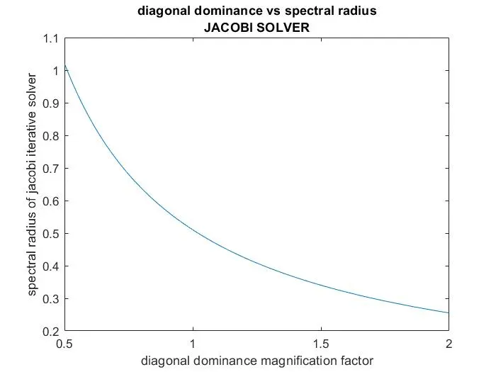
With increase in magnification factor, the spectral radius decreases from 1.0204 to 0.2551. with higher magnification factor, the spectral values reaches more stable solution.

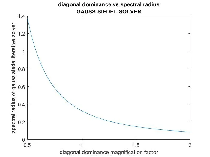
A similar trend is observed for gauss seidel solver, where the stability of spectral radius is reached when decreasing from 1.3815 to 0.0859

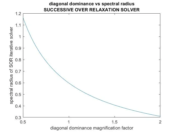
In this case also for SOR solver, the spectral radius decreases from 1.1633 to 0.3095 with increase in magnification factor. The rate of decreasing is much faster than jacobi or gauss siedel solver.

• no of iteration vs spectral radius

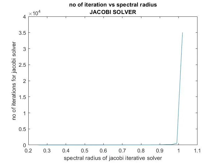
With decrease in no of iteration from 35025 to 8, the spectral radius is also found to decrease from 1.0204 to 0.2551. for the highest iteration value, the spectral radius is higher than 1, which implies instability in solution.

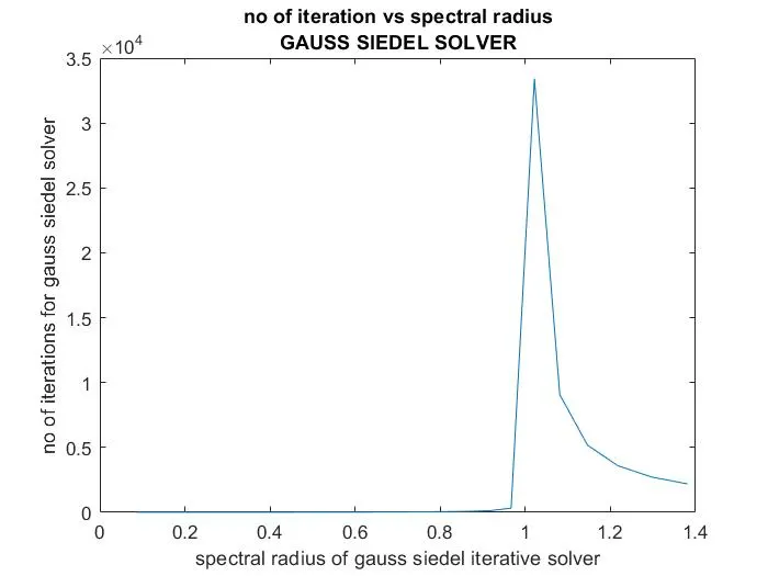
In gauss seidel solver the no of iteration rises up from 2189 to 9067 and then decreases to 6. The rise in iteration signifies instability and fluctuation in solution. As table solution of spectral radius is achieved from 0.966. above this value of spectral radius, the solution become unstable in nature.

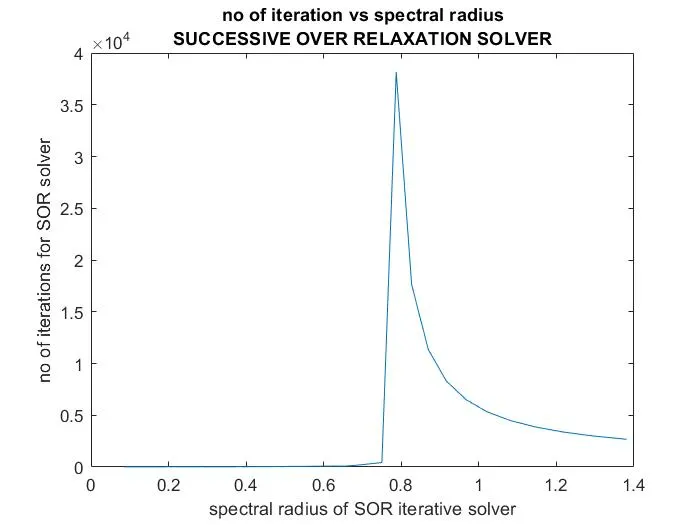
The similar nature of curve is obtained in SOR solver. The iteration rises from 2676 to 17612 and then decreases to 9. The spectral radius decreases from 1.1633 to 0.3095. the stability of spectral radius rises from 0.8811. from 1.1633 to 0.9008 the solution becomes unstable.

• no of iteration vs diagonal dominance

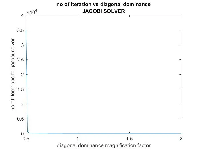
The curve is decreasing with the fall in the no of iterations and increasing magnification factor. The solution reaches a stable state at higher magnification factor.

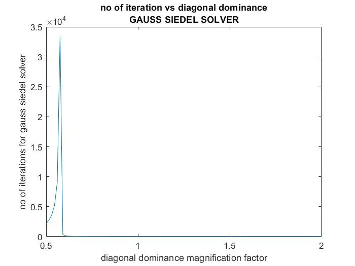
In between 0.5-1 of magnification factor, the no of iteration rises sharply and then decreases faster to achieve a stable result. The rise in iteration results in an unstable solution.

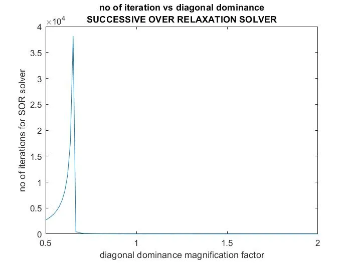
In this case also the no of iteration increases at first and then rapidly falls down with increasing magnitude of magnification factor. At higher magnification factor it gives a stable solution.

• characteristic roots vs spectral radius

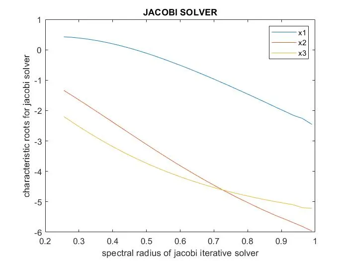
The spectral radius varies from 1.0204 to 0.2551, the values of x1 (-2.4553 to 0.426), x2 (-5.96 to -1.37), x3 (-5.215 to -2.196). With change in no of iteration the new values of x1, x2, x3 gets updated. Beyond these values unstable solution gets produced.

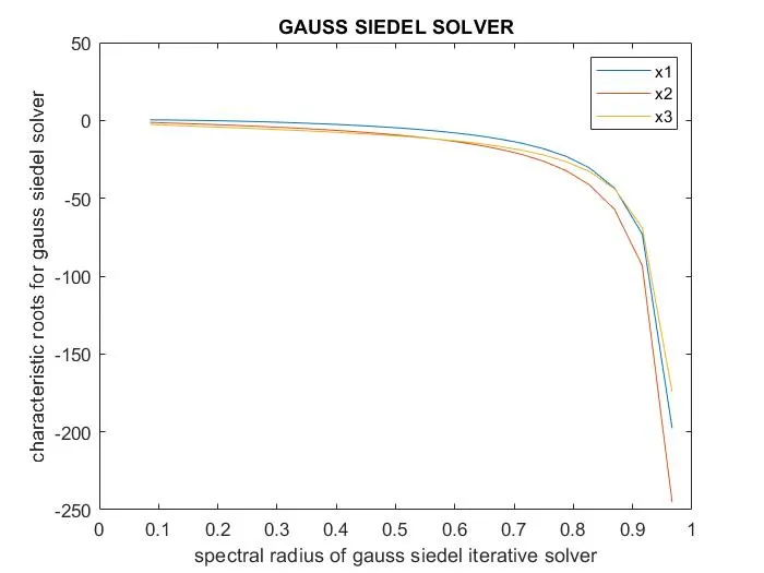
The spectral radius gives stable results within the range (0.966 to 0.2551). the values of x1 (-197.62 to 0.37), x2 (-245.23 to -1.2745), x3 (-174.32 to -2.512). the maximum value of spectral radius is close to 1. Beyond these spectral radius value, the x1, x2, x3 gets unstable.

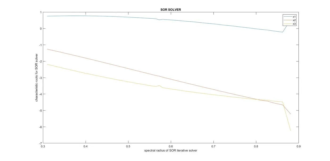
The spectral radius gives stable results within the range (0.8811 to 0.3095). the values of x1 (0.53 to 0.74), x2 (-5.218 to -1.257), x3 (-6.2426 to -2.183). the maximum value of spectral radius is close to 1. Beyond these spectral radius (0.8811) value, the x1, x2, x3 gets unstable.

comparison between computed and analytical spectral radius

• JACOBI SOLVER

• GAUSS SIEDEL SOLVER

• SOR SOLVER

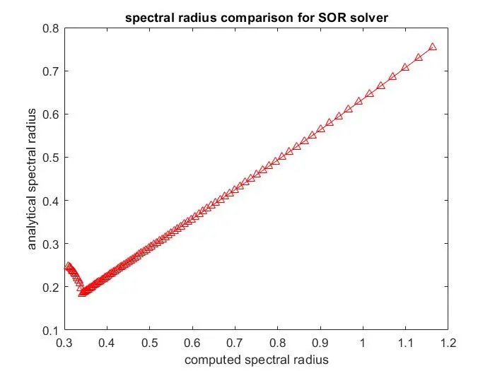
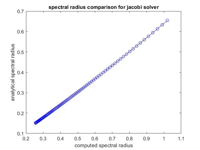
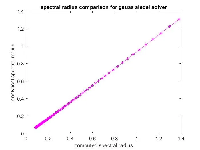
from the above comparison we see that the analytical spectral radius value matches almost close to computational values of spectral radius. This represents a perfect straight line fit in between the two values, and also very less deviation of errors.

Output

rho_j'          

    1.0204
    0.9904
    0.9621
    0.9354
    0.9101
    0.8862
    0.8634
    0.8418
    0.8213
    0.8018
    0.7831
    0.7653
    0.7483
    0.7320
    0.7165
    0.7015
    0.6872
    0.6735
    0.6603
    0.6476
    0.6354
    0.6236
    0.6122
    0.6013
    0.5908
    0.5806
    0.5707
    0.5612
    0.5520
    0.5431
    0.5345
    0.5262
    0.5181
    0.5102
    0.5026
    0.4952
    0.4880
    0.4811
    0.4743
    0.4677
    0.4613
    0.4551
    0.4490
    0.4431
    0.4373
    0.4317
    0.4262
    0.4209
    0.4157
    0.4107
    0.4057
    0.4009
    0.3962
    0.3916
    0.3871
    0.3827
    0.3784
    0.3742
    0.3700
    0.3660
    0.3621
    0.3582
    0.3545
    0.3508
    0.3472
    0.3436
    0.3401
    0.3367
    0.3334
    0.3301
    0.3269
    0.3238
    0.3207
    0.3177
    0.3147
    0.3118
    0.3089
    0.3061
    0.3034
    0.3007
    0.2980
    0.2954
    0.2928
    0.2903
    0.2878
    0.2854
    0.2830
    0.2806
    0.2783
    0.2760
    0.2738
    0.2716
    0.2694
    0.2673
    0.2651
    0.2631
    0.2610
    0.2590
    0.2571
    0.2551

rho_gs'

    1.3815
    1.2954
    1.2172
    1.1460
    1.0809
    1.0213
    0.9666
    0.9162
    0.8697
    0.8267
    0.7869
    0.7500
    0.7157
    0.6837
    0.6538
    0.6259
    0.5998
    0.5754
    0.5524
    0.5308
    0.5105
    0.4914
    0.4733
    0.4563
    0.4402
    0.4249
    0.4105
    0.3968
    0.3838
    0.3714
    0.3596
    0.3485
    0.3378
    0.3276
    0.3180
    0.3087
    0.2999
    0.2914
    0.2833
    0.2756
    0.2682
    0.2610
    0.2542
    0.2477
    0.2414
    0.2353
    0.2295
    0.2239
    0.2185
    0.2134
    0.2084
    0.2036
    0.1989
    0.1944
    0.1901
    0.1860
    0.1819
    0.1780
    0.1743
    0.1706
    0.1671
    0.1637
    0.1604
    0.1572
    0.1541
    0.1511
    0.1481
    0.1453
    0.1426
    0.1399
    0.1373
    0.1348
    0.1324
    0.1300
    0.1277
    0.1255
    0.1233
    0.1212
    0.1191
    0.1171
    0.1151
    0.1132
    0.1114
    0.1096
    0.1078
    0.1061
    0.1044
    0.1028
    0.1012
    0.0996
    0.0981
    0.0966
    0.0952
    0.0938
    0.0924
    0.0910
    0.0897
    0.0884
    0.0872
    0.0859


rho_sor'

    1.1633
    1.1301
    1.0988
    1.0693
    1.0414
    1.0149
    0.9897
    0.9659
    0.9431
    0.9215
    0.9008
    0.8811
    0.8623
    0.8442
    0.8270
    0.8104
    0.7945
    0.7793
    0.7646
    0.7505
    0.7369
    0.7239
    0.7113
    0.6991
    0.6874
    0.6760
    0.6651
    0.6545
    0.6443
    0.6343
    0.6247
    0.6154
    0.6064
    0.5976
    0.5891
    0.5809
    0.5728
    0.5650
    0.5575
    0.5501
    0.5429
    0.5360
    0.5292
    0.5225
    0.5161
    0.5098
    0.5037
    0.4977
    0.4919
    0.4862
    0.4806
    0.4752
    0.4699
    0.4647
    0.4596
    0.4547
    0.4498
    0.4451
    0.4404
    0.4359
    0.4314
    0.4271
    0.4228
    0.4187
    0.4146
    0.4106
    0.4066
    0.4028
    0.3990
    0.3953
    0.3917
    0.3881
    0.3846
    0.3811
    0.3778
    0.3744
    0.3712
    0.3680
    0.3649
    0.3618
    0.3587
    0.3557
    0.3528
    0.3499
    0.3471
    0.3443
    0.3416
    0.3389
    0.3362
    0.3336
    0.3310
    0.3285
    0.3260
    0.3235
    0.3211
    0.3187
    0.3164
    0.3141
    0.3118
    0.3095

%%%%%jacobi solver%%%%
x1_j'
   -Inf
   -2.4553
   -2.2595
   -2.1565
   -2.0254
   -1.9042
   -1.7849
   -1.6728
   -1.5669
   -1.4677
   -1.3739
   -1.2849
   -1.2006
   -1.1204
   -1.0453
   -0.9724
   -0.9046
   -0.8401
   -0.7789
   -0.7211
   -0.6656
   -0.6130
   -0.5629
   -0.5154
   -0.4730
   -0.4294
   -0.3881
   -0.3488
   -0.3115
   -0.2761
   -0.2423
   -0.2102
   -0.1797
   -0.1506
   -0.1228
   -0.0964
   -0.0712
   -0.0472
   -0.0243
   -0.0025
    0.0184
    0.0383
    0.0573
    0.0754
    0.0927
    0.1093
    0.1251
    0.1401
    0.1545
    0.1682
    0.1813
    0.1938
    0.2058
    0.2172
    0.2280
    0.2385
    0.2485
    0.2580
    0.2671
    0.2758
    0.2841
    0.2921
    0.2997
    0.3069
    0.3122
    0.3189
    0.3253
    0.3315
    0.3373
    0.3429
    0.3482
    0.3533
    0.3581
    0.3627
    0.3671
    0.3713
    0.3753
    0.3791
    0.3827
    0.3861
    0.3894
    0.3925
    0.3954
    0.3982
    0.4009
    0.4034
    0.4057
    0.4080
    0.4101
    0.4122
    0.4141
    0.4159
    0.4176
    0.4191
    0.4206
    0.4220
    0.4234
    0.4246
    0.4257
    0.4268

x2_j'
 NaN
   -5.9624
   -5.8137
   -5.6880
   -5.5724
   -5.4669
   -5.3548
   -5.2487
   -5.1417
   -5.0356
   -4.9364
   -4.8383
   -4.7419
   -4.6474
   -4.5557
   -4.4654
   -4.3775
   -4.2918
   -4.2082
   -4.1269
   -4.0475
   -3.9703
   -3.8961
   -3.8225
   -3.7533
   -3.6831
   -3.6149
   -3.5486
   -3.4841
   -3.4214
   -3.3604
   -3.3010
   -3.2432
   -3.1869
   -3.1321
   -3.0787
   -3.0267
   -2.9760
   -2.9267
   -2.8786
   -2.8317
   -2.7861
   -2.7415
   -2.6981
   -2.6558
   -2.6143
   -2.5740
   -2.5347
   -2.4964
   -2.4590
   -2.4225
   -2.3869
   -2.3521
   -2.3181
   -2.2849
   -2.2525
   -2.2208
   -2.1898
   -2.1596
   -2.1300
   -2.1011
   -2.0729
   -2.0452
   -2.0182
   -1.9923
   -1.9664
   -1.9410
   -1.9162
   -1.8920
   -1.8682
   -1.8449
   -1.8222
   -1.7999
   -1.7780
   -1.7566
   -1.7357
   -1.7151
   -1.6950
   -1.6753
   -1.6559
   -1.6370
   -1.6184
   -1.6001
   -1.5822
   -1.5647
   -1.5475
   -1.5306
   -1.5140
   -1.4978
   -1.4818
   -1.4661
   -1.4508
   -1.4356
   -1.4208
   -1.4062
   -1.3919
   -1.3779
   -1.3641
   -1.3505
   -1.3371

x3_j'

 Inf
   -5.2159
   -5.1949
   -5.1001
   -5.0501
   -5.0035
   -4.9562
   -4.9109
   -4.8634
   -4.8141
   -4.7682
   -4.7218
   -4.6753
   -4.6291
   -4.5827
   -4.5377
   -4.4916
   -4.4461
   -4.4010
   -4.3560
   -4.3120
   -4.2684
   -4.2261
   -4.1831
   -4.1395
   -4.0978
   -4.0567
   -4.0160
   -3.9758
   -3.9360
   -3.8968
   -3.8582
   -3.8200
   -3.7823
   -3.7452
   -3.7086
   -3.6725
   -3.6369
   -3.6018
   -3.5672
   -3.5331
   -3.4996
   -3.4665
   -3.4340
   -3.4019
   -3.3701
   -3.3390
   -3.3083
   -3.2780
   -3.2482
   -3.2189
   -3.1900
   -3.1615
   -3.1335
   -3.1057
   -3.0785
   -3.0517
   -3.0253
   -2.9993
   -2.9736
   -2.9484
   -2.9235
   -2.8989
   -2.8748
   -2.8496
   -2.8262
   -2.8032
   -2.7805
   -2.7581
   -2.7360
   -2.7142
   -2.6928
   -2.6716
   -2.6507
   -2.6301
   -2.6098
   -2.5898
   -2.5701
   -2.5506
   -2.5314
   -2.5125
   -2.4938
   -2.4753
   -2.4572
   -2.4392
   -2.4215
   -2.4040
   -2.3868
   -2.3698
   -2.3530
   -2.3364
   -2.3201
   -2.3039
   -2.2880
   -2.2722
   -2.2567
   -2.2414
   -2.2262
   -2.2113
   -2.1965

%%%%%gauss siedel solver%%%

x1_gs'

      -Inf
      -Inf
      -Inf
      -Inf
      -Inf
      -Inf
 -197.6239
  -73.0278
  -43.5638
  -30.4119
  -22.9807
  -18.2158
  -14.9083
  -12.4837
  -10.6341
   -9.1798
   -8.0088
   -7.0473
   -6.2455
   -5.5676
   -4.9883
   -4.4882
   -4.0530
   -3.6712
   -3.3343
   -3.0352
   -2.7682
   -2.5289
   -2.3133
   -2.1185
   -1.9419
   -1.7810
   -1.6342
   -1.4999
   -1.3767
   -1.2633
   -1.1588
   -1.0624
   -0.9731
   -0.8904
   -0.8135
   -0.7421
   -0.6756
   -0.6135
   -0.5556
   -0.5015
   -0.4507
   -0.4032
   -0.3587
   -0.3169
   -0.2776
   -0.2406
   -0.2058
   -0.1730
   -0.1421
   -0.1130
   -0.0854
   -0.0594
   -0.0348
   -0.0116
    0.0104
    0.0312
    0.0509
    0.0696
    0.0873
    0.1041
    0.1201
    0.1352
    0.1496
    0.1632
    0.1762
    0.1886
    0.2003
    0.2114
    0.2220
    0.2321
    0.2417
    0.2508
    0.2595
    0.2677
    0.2756
    0.2831
    0.2902
    0.2970
    0.3034
    0.3096
    0.3154
    0.3210
    0.3263
    0.3313
    0.3361
    0.3407
    0.3450
    0.3492
    0.3531
    0.3568
    0.3604
    0.3638
    0.3670
    0.3700

x2_gs'

      -Inf
      -Inf
      -Inf
      -Inf
      -Inf
      -Inf
 -245.2317
  -93.3225
  -57.3469
  -41.2521
  -32.1308
  -26.2608
  -22.1687
  -19.1544
  -16.8426
  -15.0140
  -13.5324
  -12.3076
  -11.2789
  -10.4027
   -9.6478
   -8.9908
   -8.4141
   -7.9038
   -7.4492
   -7.0419
   -6.6748
   -6.3424
   -6.0399
   -5.7638
   -5.5106
   -5.2775
   -5.0626
   -4.8636
   -4.6789
   -4.5070
   -4.3467
   -4.1969
   -4.0566
   -3.9249
   -3.8010
   -3.6843
   -3.5743
   -3.4703
   -3.3719
   -3.2787
   -3.1902
   -3.1061
   -3.0262
   -2.9501
   -2.8775
   -2.8083
   -2.7422
   -2.6789
   -2.6184
   -2.5604
   -2.5048
   -2.4514
   -2.4002
   -2.3510
   -2.3037
   -2.2582
   -2.2143
   -2.1721
   -2.1313
   -2.0920
   -2.0541
   -2.0175
   -1.9820
   -1.9478
   -1.9146
   -1.8825
   -1.8515
   -1.8214
   -1.7922
   -1.7639
   -1.7365
   -1.7099
   -1.6840
   -1.6589
   -1.6345
   -1.6108
   -1.5877
   -1.5652
   -1.5434
   -1.5221
   -1.5014
   -1.4812
   -1.4616
   -1.4424
   -1.4237
   -1.4055
   -1.3877
   -1.3704
   -1.3535
   -1.3369
   -1.3208
   -1.3050
   -1.2895
   -1.2745


x3_gs'

-Inf
      -Inf
      -Inf
      -Inf
      -Inf
      -Inf
 -174.3288
  -68.9872
  -43.9826
  -32.7567
  -26.3654
  -22.2295
  -19.3277
  -17.1748
  -15.5109
  -14.1837
  -13.0987
  -12.1935
  -11.4258
  -10.7654
  -10.1907
   -9.6852
   -9.2368
   -8.8357
   -8.4746
   -8.1474
   -7.8493
   -7.5764
   -7.3254
   -7.0936
   -6.8788
   -6.6790
   -6.4926
   -6.3182
   -6.1545
   -6.0006
   -5.8556
   -5.7186
   -5.5889
   -5.4660
   -5.3492
   -5.2380
   -5.1322
   -5.0312
   -4.9346
   -4.8423
   -4.7538
   -4.6690
   -4.5875
   -4.5093
   -4.4340
   -4.3615
   -4.2917
   -4.2243
   -4.1593
   -4.0965
   -4.0357
   -3.9770
   -3.9201
   -3.8651
   -3.8117
   -3.7599
   -3.7097
   -3.6609
   -3.6135
   -3.5675
   -3.5227
   -3.4791
   -3.4367
   -3.3954
   -3.3552
   -3.3160
   -3.2778
   -3.2405
   -3.2042
   -3.1687
   -3.1340
   -3.1002
   -3.0671
   -3.0348
   -3.0032
   -2.9724
   -2.9421
   -2.9126
   -2.8836
   -2.8553
   -2.8276
   -2.8004
   -2.7738
   -2.7477
   -2.7221
   -2.6971
   -2.6725
   -2.6484
   -2.6247
   -2.6015
   -2.5787
   -2.5563
   -2.5343
   -2.5128

%%%%%%SOR solver%%%%%%

x1_sor'
Inf
       NaN
      -Inf
       Inf
      -Inf
      -Inf
      -Inf
       Inf
       Inf
       Inf
      -Inf
    0.5304
   -0.2234
   -0.1625
   -0.0967
   -0.0541
   -0.0023
    0.0475
    0.0912
    0.1349
    0.1743
    0.2095
    0.2483
    0.2842
    0.3133
    0.3434
    0.3705
    0.4027
    0.4226
    0.4459
    0.4690
    0.4894
    0.5089
    0.5274
    0.5450
    0.5613
    0.5306
    0.5908
    0.6045
    0.6173
    0.6294
    0.6406
    0.6510
    0.6610
    0.6703
    0.6795
    0.6881
    0.6952
    0.7024
    0.7090
    0.7152
    0.7210
    0.7264
    0.7313
    0.7361
    0.7403
    0.7442
    0.7479
    0.7515
    0.7545
    0.7572
    0.7593
    0.7632
    0.7642
    0.7656
    0.7672
    0.7687
    0.7693
    0.7781
    0.7719
    0.7727
    0.7733
    0.7737
    0.7740
    0.7742
    0.7742
    0.7742
    0.7740
    0.7737
    0.7733
    0.7726
    0.7721
    0.7714
    0.7707
    0.7699
    0.7690
    0.7680
    0.7669
    0.7658
    0.7647
    0.7634
    0.7621
    0.7607
    0.7593
    0.7579
    0.7564
    0.7550
    0.7535
    0.7514
    0.7498

x2_sor'
NaN
       NaN
       NaN
       NaN
       NaN
       NaN
       NaN
       NaN
       NaN
       NaN
       NaN
   -5.2180
   -4.6598
   -4.5619
   -4.4337
   -4.3728
   -4.2832
   -4.1950
   -4.1111
   -4.0274
   -3.9474
   -3.8674
   -3.7923
   -3.7102
   -3.6460
   -3.5757
   -3.5084
   -3.4368
   -3.3769
   -3.3150
   -3.2523
   -3.1933
   -3.1356
   -3.0794
   -3.0248
   -2.9707
   -2.9059
   -2.8693
   -2.8201
   -2.7723
   -2.7257
   -2.6803
   -2.6360
   -2.5929
   -2.5517
   -2.5098
   -2.4696
   -2.4311
   -2.3932
   -2.3563
   -2.3202
   -2.2850
   -2.2506
   -2.2171
   -2.1844
   -2.1524
   -2.1213
   -2.0908
   -2.0611
   -2.0320
   -2.0036
   -1.9760
   -1.9490
   -1.9212
   -1.8963
   -1.8709
   -1.8460
   -1.8224
   -1.7995
   -1.7748
   -1.7520
   -1.7298
   -1.7080
   -1.6866
   -1.6658
   -1.6453
   -1.6254
   -1.6057
   -1.5865
   -1.5676
   -1.5491
   -1.5310
   -1.5132
   -1.4958
   -1.4787
   -1.4620
   -1.4456
   -1.4295
   -1.4137
   -1.3981
   -1.3829
   -1.3680
   -1.3537
   -1.3393
   -1.3252
   -1.3113
   -1.2974
   -1.2840
   -1.2708
   -1.2578

x3_sor'

       NaN
      -Inf
       NaN
       NaN
       NaN
       NaN
       NaN
       NaN
       NaN
       NaN
       NaN
   -6.2426
   -4.4765
   -4.4355
   -4.3738
   -4.3484
   -4.3101
   -4.2727
   -4.2321
   -4.1937
   -4.1541
   -4.1093
   -4.0774
   -4.0344
   -4.0011
   -3.9640
   -3.9261
   -3.8934
   -3.8535
   -3.8183
   -3.7826
   -3.7470
   -3.7122
   -3.6778
   -3.6445
   -3.6098
   -3.4740
   -3.5444
   -3.5121
   -3.4803
   -3.4490
   -3.4177
   -3.3866
   -3.3565
   -3.3278
   -3.2980
   -3.2694
   -3.2404
   -3.2122
   -3.1844
   -3.1570
   -3.1299
   -3.1032
   -3.0768
   -3.0512
   -3.0256
   -3.0004
   -2.9755
   -2.9517
   -2.9274
   -2.9035
   -2.8792
   -2.8600
   -2.8327
   -2.8106
   -2.7883
   -2.7664
   -2.7442
   -2.7433
   -2.7024
   -2.6817
   -2.6612
   -2.6410
   -2.6211
   -2.6014
   -2.5820
   -2.5630
   -2.5441
   -2.5255
   -2.5071
   -2.4885
   -2.4706
   -2.4529
   -2.4355
   -2.4183
   -2.4013
   -2.3846
   -2.3680
   -2.3517
   -2.3355
   -2.3196
   -2.3039
   -2.2888
   -2.2734
   -2.2582
   -2.2432
   -2.2282
   -2.2136
   -2.1974
   -2.1832

Conclusions:

• The spectral radius is seen to decrease with increase in magnification factor. The rate of decrease in spectral radius is faster for SOR solver, which indicates the stability of the system even at higher spectral values.
• With decrease in no of iteration for three solvers, it is seen that the spectral radius also decreases. At a very high spectral radius value (ρ>1) the values of x1, x2 and x3 gets unstable and fluctuates. With low values of ρ a stable solution is attained.
• With increase in magnification factor, the no of iterations falls down drastically. The slope for decreasing is highest for Jacobi solver and lowest for SOR solver.