Week 6: Conjugate Heat Transfer Simulation
Abstract:
In this project, a conjugate heat transfer simulation of a pipe flow is studied. Following a baseline mesh, grid independency test has been done at different supercycling interval. Post processing and data comparison is carried out using Paraview tool.
Aim:
Conjugate heat transfer simulation of a pipe.
Objective:
- Setup a flow simulation through a pipe
- Inlet Reynolds number should be 7,000
-
HINT : Use the below formula to calculate velocity for corresponding value of REYNOLD NUMBER and give DIRICHLET BC for velocity at inlet and specify the value for velocity calculated at INLET BC using below formula ,
Re = (rho*V*D)/(Dynamic viscosity)
-
- Turbulence modelling - K-Epsilon
- Supercycling parameters - same as in the video
Additional 3D outputs
- Add Y+ to your post.in file
Grid dependence test
- Start with an initial base grid
- Run grid dependence test on 3 grids and show that the outlet temperature converges to a particular value
Effect of supercycle stage interval
- Set supercyle stage interval to 0.01,0.02 and 0.03
- For these three values, how does the total simulation time compare against the baseline configuration
Theory:
Conjugate heat transfer allows simulation of heat transfer between solid and fluid domain by exchanging thermal energies at the interface between them. Some typical turbulence model is used in modelling CHT are laminar, RANS, LES. In solids conduction often dominates and in fluids, convection usually dominates. Efficiently combining heat transfer in solid and fluid is the key to design effective coolers, heaters and heat exchangers. Heat transfer in solid and fluid are combined in a majority of application. Typical application of CHT can be performed to improve cooling performance of water jacket and increase engine life. Advancements in cooling for application in gas turbine to understand the complex heat transfer interactions. Critical cooling application involves internal and external film cooling. CHT analysis provides thermal distribution in solid and coolant of engine to provide better insight in velocity distribution and designing thermal load capacity.
Heat Transfer by Solids and Fluids
Heat Transfer in a Solid
In most cases, heat transfer in solids, if only due to conduction, is described by Fourier’s law defining the conductive heat flux, q, proportional to the temperature gradient: .
For a time-dependent problem, the temperature field in an immobile solid verifies the following form of the heat equation:
Heat Transfer in a Fluid
Due to the fluid motion, three contributions to the heat equation are included:
- The transport of fluid implies energy transport too, which appears in the heat equation as the convective contribution. Depending on the thermal properties on the fluid and on the flow regime, either the convective or the conductive heat transfer can dominate.
- The viscous effects of the fluid flow produce fluid heating. This term is often neglected, nevertheless, its contribution is noticeable for fast flow in viscous fluids.
- As soon as a fluid density is temperature-dependent, a pressure work term contributes to the heat equation. This accounts for the well-known effect that, for example, compressing air produces heat.
Conjugate Heat Transfer Applications
Effective Heat Transfer
Efficiently combining heat transfer in fluids and solids is the key to designing effective coolers, heaters, or heat exchangers.
The fluid usually plays the role of energy carrier on large distances. Forced convection is the most common way to achieve high heat transfer rate. In some applications, the performances are further improved by combining convection with phase change (for example liquid water to vapor phase change).
Even so, solids are also needed, in particular to separate fluids in a heat exchanger so that fluids exchange energy without being mixed.
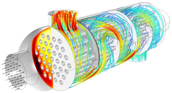
Flow and temperature field in a shell-and-tube heat exchanger illustrating heat transfer between two fluids separated by the thin metallic wall.
Heat sinks are usually made of metal with high thermal conductivity (e.g. copper or aluminum). They dissipate heat by increasing the exchange area between the solid part and the surrounding fluid.
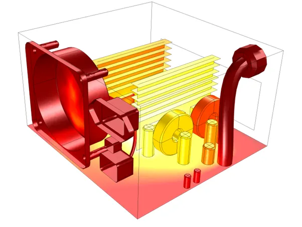
Energy Savings
Heat transfer in fluids and solids can also be combined to minimize heat losses in various devices. Because most gases (especially at low pressure) have small thermal conductivities, they can be used as thermal insulators… provided they are not in motion. In many situations, gas is preferred to other material due to its low weight. In any case, it is important to limit the heat transfer by convection, in particular by reducing the natural convection effects. Judicious positioning of walls and use of small cavities helps to control the natural convection. Applied at the micro scale, the principle leads to the insulation foam concept where tiny cavities of air (bubbles) are trapped in the foam material (e.g. polyurethane), which combines high insulation performances with light weight.
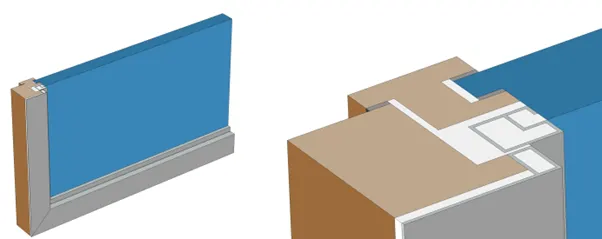
Window cross section (left) and zoom-in on the window frame (right).
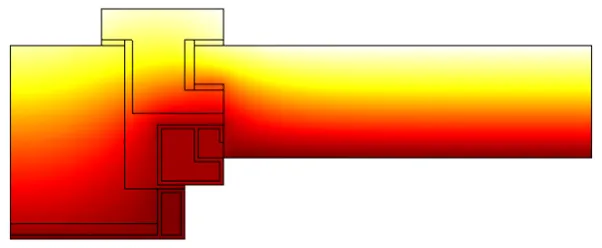
Temperature profile in a window frame and glazing cross section from ISO 10077-2:2012 (thermal performance of windows).
Fluid and Solid Interactions
Fluid/Solid Interface
The temperature field and the heat flux are continuous at the fluid/solid interface. However, the temperature field can rapidly vary in a fluid in motion: close to the solid, the fluid temperature is close to the solid temperature, and far from the interface, the fluid temperature is close to the inlet or ambient fluid temperature. The distance where the fluid temperature varies from the solid temperature to the fluid bulk temperature is called the thermal boundary layer. The thermal boundary layer size and the momentum boundary layer relative size is reflected by the Prandtl number : for the Prandtl number to equal 1, thermal and momentum boundary layer thicknesses need to be the same. A thicker momentum layer would result in a Prandtl number larger than 1. Conversely, a Prandtl number smaller than 1 would indicate that the momentum boundary layer is thinner than the thermal boundary layer. The Prandtl number for air at atmospheric pressure and at 20°C is 0.7. That is because for air, the momentum and thermal boundary layer have similar size, while the momentum boundary layer is slightly thinner than the thermal boundary layer. For water at 20°C, the Prandtl number is about 7. So, in water, the temperature changes close to a wall are sharper than the velocity change.
The fluid flow and heat transfer problems can be tightly coupled through the convection term in the energy equation and when physical properties are temperature dependent. While analytical solutions exist for some simple problems, we must rely on computational methods to solve most industrially relevant applications.
CHT can be performed to improve cooling performance of the water jacket and increase engine life. Advancements in cooling for applications such as gas turbines components require improved understanding of the complex heat transfer mechanisms and the interactions between those mechanisms, which our engineers can perform without hassle. Critical cooling applications often rely on multiple thermal protection techniques, including internal cooling, external film cooling, etc. which are efficiently used by our analysis to cool components and limit the use of coolant. We do extensive support for Motor and Battery CHT Analysis to get optimized design for High voltage systems. Conjugate Heat Transfer analysis provides the temperature distribution in solid and coolant of the engine and clear insight on velocity distribution and mechanism of heat transfer of coolant. Results of CHT analysis become input to structural simulations as thermal loads.
We have a wide experience in Engine CHT Analysis for various type of engines like Bikes, Passenger Cars, Racing cars, Commercial Vehicles, Marine, Agricultural equipment and Earth-moving equipment etc.
Geometrical creation:
Open the converge panel
go to create>> select shape>> select cylinder
outer cylinder radius: 0.015
length 0.2m
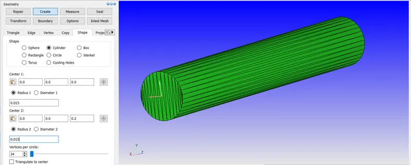
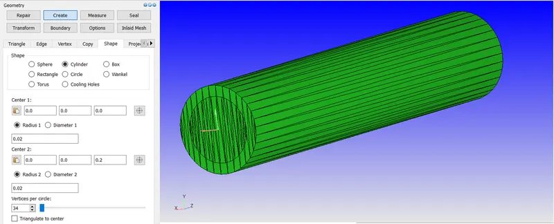
create inner cylinder with radius 0.02
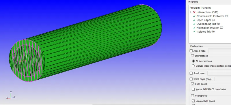
check on the diagnosis tab, intersection and manifold errors will be seen
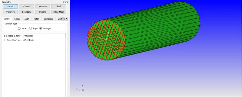
to clean the intersection error
select the interfacing triangles and delete them
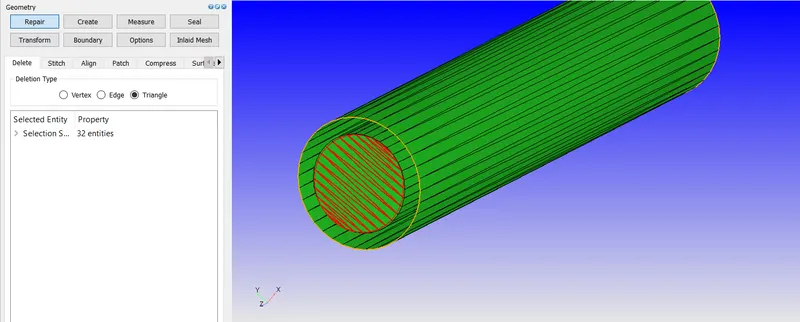
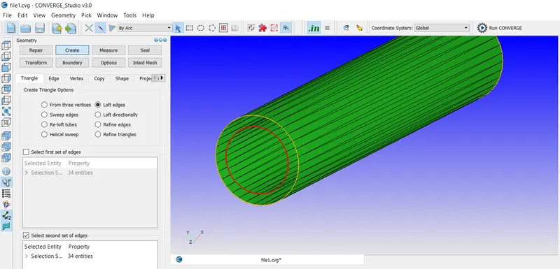
To remove the open edge problem, we loft the inner and outer extreme edges of the cylinder.
enable the edge selection option with by arc option>> go to create>> select triangles>> select loft edges>> select first and second sets of edges
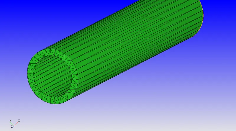
now we use patch tool to create the inlet and outlet faces of the cylinder
go to repair>> select list of edges option>> enable the edge selection tab with by arc option>> select the list of edges option>> select the inlet edge
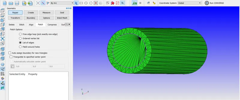
The same procedure for the outlet is repeated
Now to check the normal, we ensure that all normals should point inwards
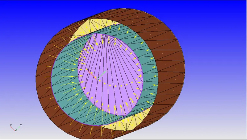
Computation of velocity and the base grid size:
Re= 7000
Density= 1.17kg/m3
Viscosity= 0.00001846
Diameter = 0.03m
`Re=ρvd/μ`
`7000=(1.17*v*0.03)/0.00001846`
v= 3.6814m/s
`ϑ=μ/ρ=0.00001846/1.177=0.000015684`
`C_f=0.00576Re^(-1/5)=0.00980399`
`τ_w=C_f (ρu^2)/2=0.07728`
`U_t=√(τ_w/ρ)=0.25631`
Assume the desired y +=32
Then the first cell thickness
`y=y+*ϑ/U_t =0.001958126m`
Cell size= 2* first cell thickness*1000= 3.962m
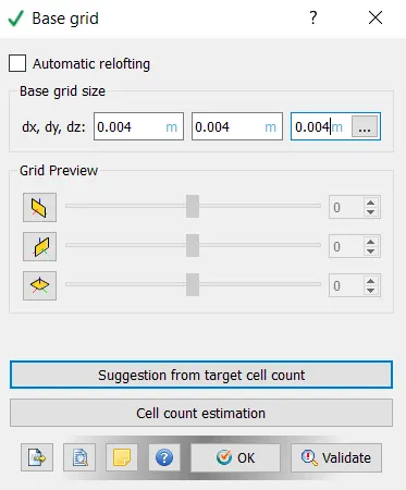
We can approximate to 4mm grid size
Simulation case set up
Open the converge 3.0 console
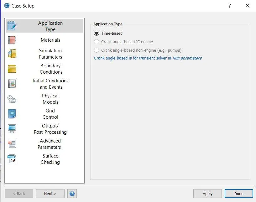
Application:
Type-time based
Materials:
Predefined mixture: air
Check gas simulation and solid simulation option and species
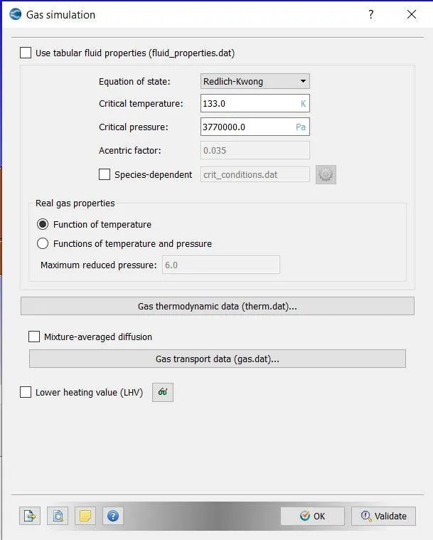
Gas simulation:
Select default parameters
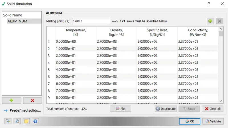
Solid simulation:
Choose predefined material: Aluminium
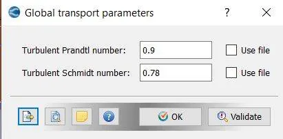
Global transport properties:
Select default settings
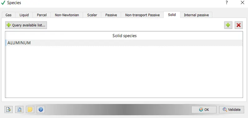
Species:
Gas –O2 and N2

Solid- Al
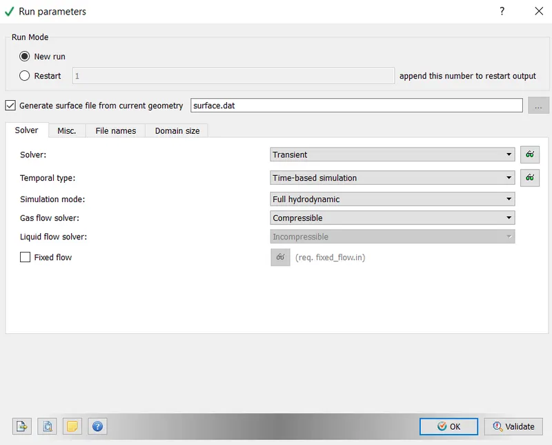
Simulation parameters:
Solver type-Transient
Simulation mode- full hydrodynamic
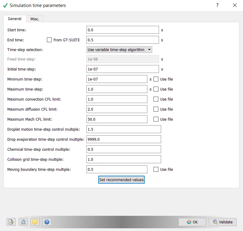
Simulation time parameters:
Start time0
End time 0.5
Initial time 1e-7
Minimum time 1e-7
Maximum time 1
Max cfl limit 1
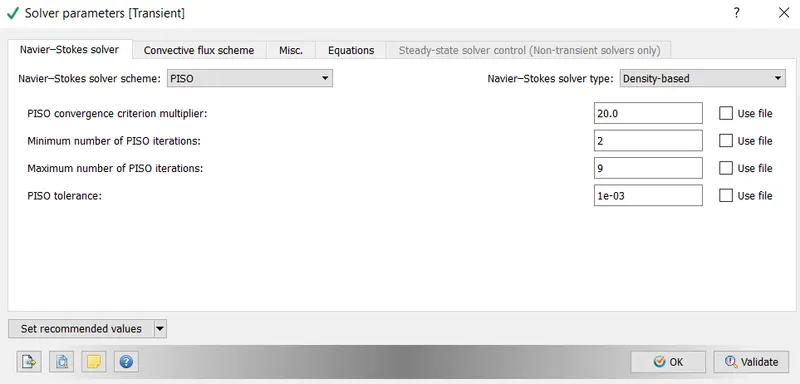
Solver parameter:
Navier-Stokes type solver- density
Boundary conditions:
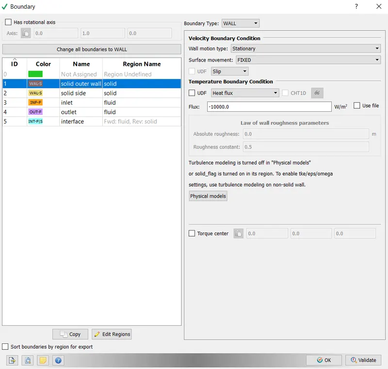
Solid outer wall:
Boundary type: wall
Wall motion type: stationary, slip
Temperature flux: -10000w/m3
Region name- solid
Solid side:
Boundary type: wall
Wall motion type: stationary, slip
Velocity: zero normal gradient
Region name-solid

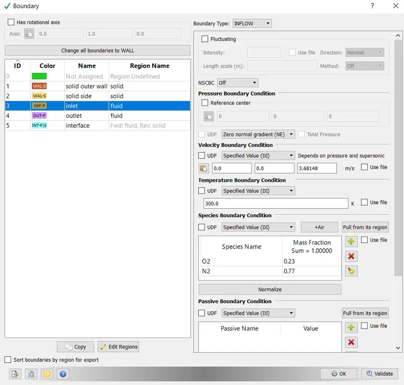
Inlet:
Boundary type: inflow
Velocity: 3.68m/s in z direction
Temperature: 300k
Species: air
Region name-fluid
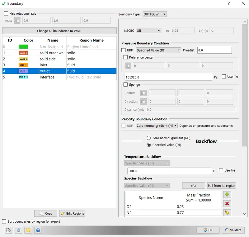
Outlet:
Boundary type: outflow
Pressure: 101325Pa
Velocity: zero normal gradient
Species backflow: air
Region name- fluid
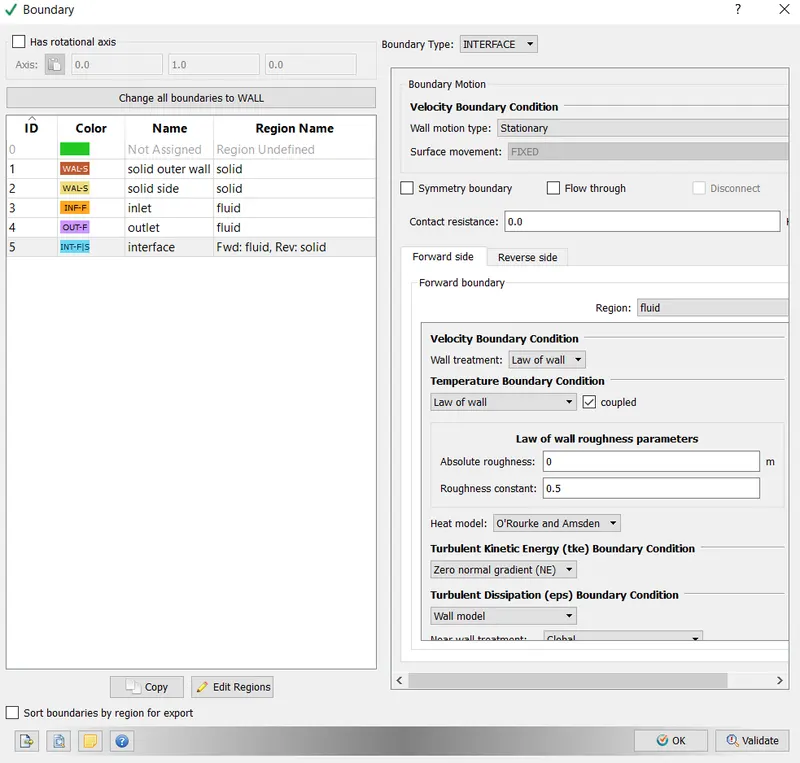
Interface:
Boundary type: interface
Forward side:
Region: fluid
Velocity: law of wall
Temperature: law of wall
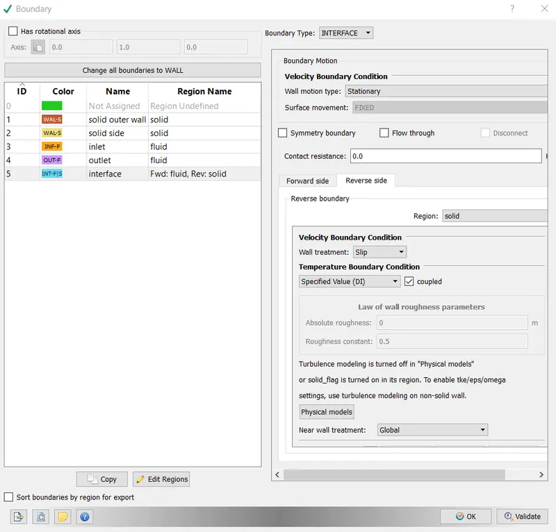
Reverse side:
Region: solid
Velocity: slip
Temperature: specified ID
Region and initialization:
Region: fluid ID-0
Temperature: 300k
Pressure: 101325
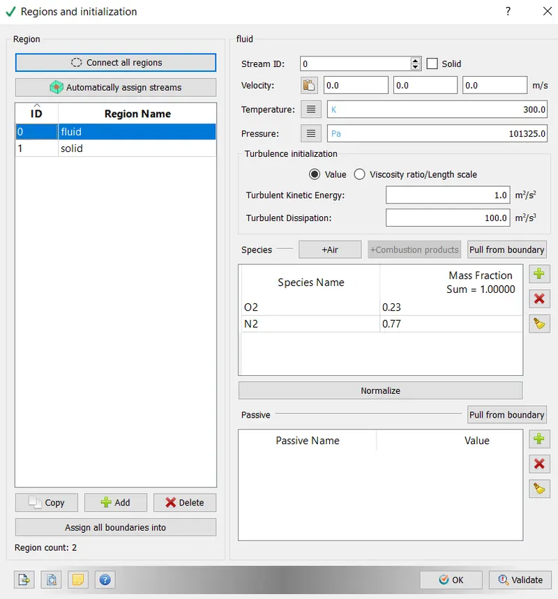
Region: solid ID-1>> check the solid option
Temperature: 300k
Species: Al
Mass fraction 1

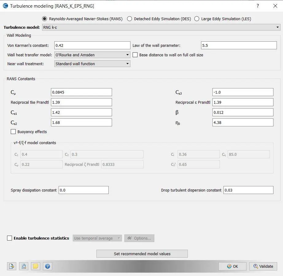
Physical model:
Enable turbulent and super cycle modelling box
Turbulent modelling: RNG k-epsilon
Super cycling:
The difference between the time scale of the solid region and fluid region is overcome by the super cycling with the basic idea that the solver for the fluid domain is paused until the solver of the solid is converged. The effect can be seen at the low cycle interval, the flow converges very early, which can be employed to solve fine mesh for reducing solver time by reducing the end time in seconds. Super cycle significantly reduces computational time and cost.
Begin starting super cycle data: 0.01
Conduction CFL limit: 100
Relaxation factor: 1.4
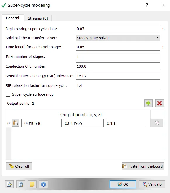
For choosing the output point
Go to measure>> select average of vertex location>> select the outlet points
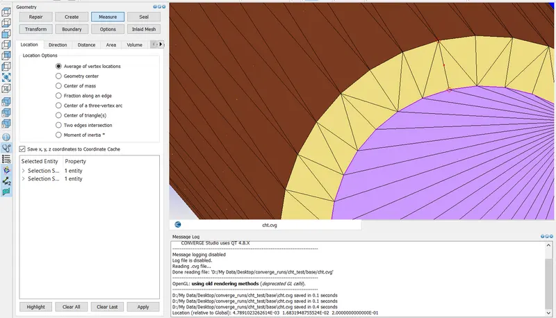
Now the outlet point is at the extreme point, it will not be able to capture the physics of heat transfer. So we push the outlet point inside the domain.
Grid control:
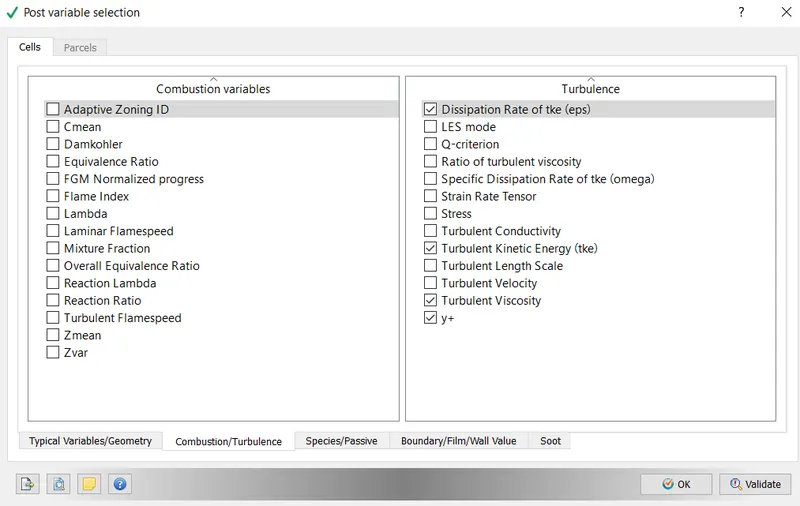
Post variable selection:
From combustion tab>> check y+
Output file processing:
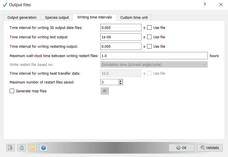
Time interval for writing 3D output files- 0.005s
Post processing:
Grid dependency test:
Case 1
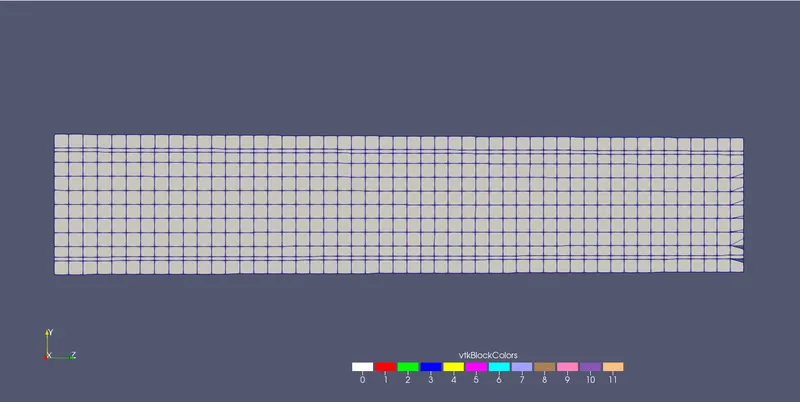
Baseline grid 0.004m
Super cycle interval: 0.005s
Mesh
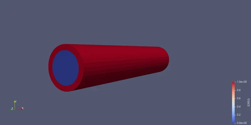
Region ID
Graphical analysis
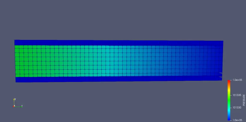
Pressure:
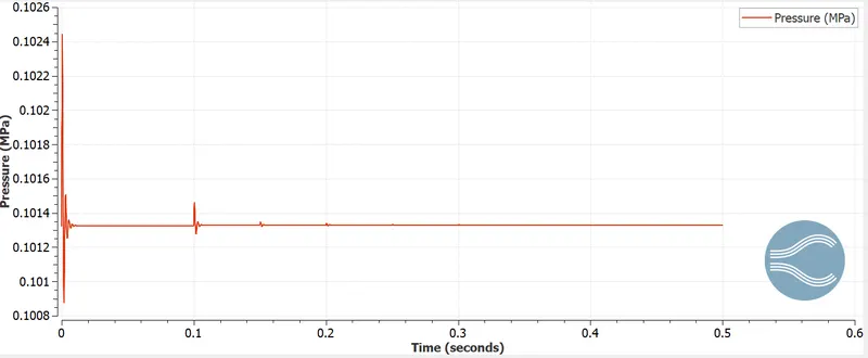
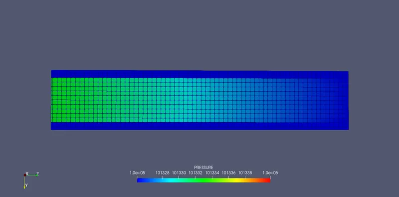
The difference between inlet and outlet pressure is measured in terms of time interval. The fluctuation of pressure is high at beginning and touches 102.4kPa and becomes steady at 101.3kPa. Initial pressure is high because of convective heat transfer from air. With increase in interval small fluctuation are to be seen due to super cycle interval at the solid and become stable gradually.
Mean temperature:
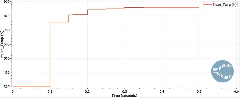
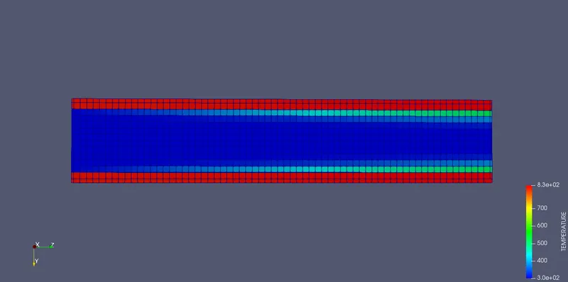
The mean temp is fluctuating with respect to time. After 0.1s the temperature shoots to 750k because of convective heat transfer at a faster rate. The solid horizontal line indicates the time taken for the solid domain to heat up.
Velocity:
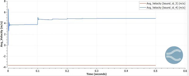
The velocity fluctuation is also a function of pressure change. Similar to pressure fluctuation, velocity is high initially as 6.5m/s and then with super cycling stages, the fluctuation reduces and become stable.
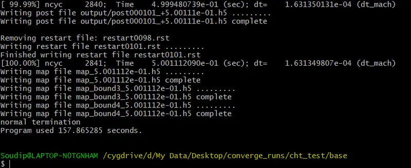
Computation time:
Contours
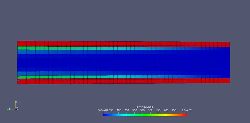
Temperature
Pressure
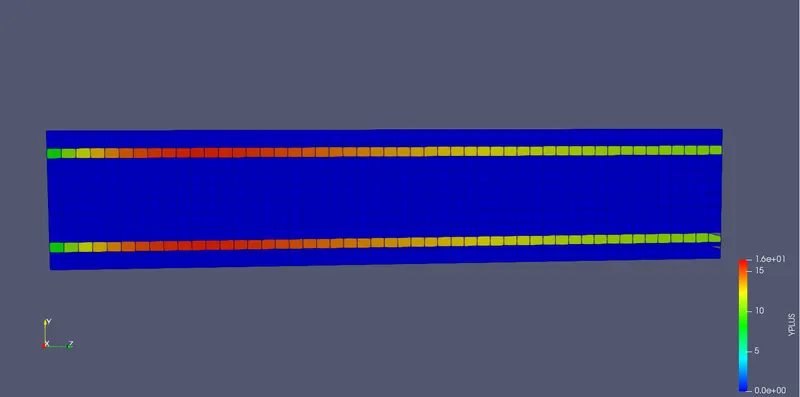
Y+ plot
cell count
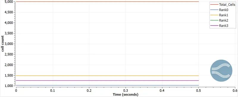
Total cell count is achieved about 5000 cells and for processor 0, 1, 2 and 3 have in between 1000-1500 cells.
Case 2
Refined grid 0.003m
Super cycle interval: 0.01s
Mesh
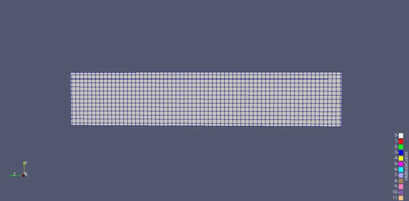
Region ID
Graphical analysis
Pressure:
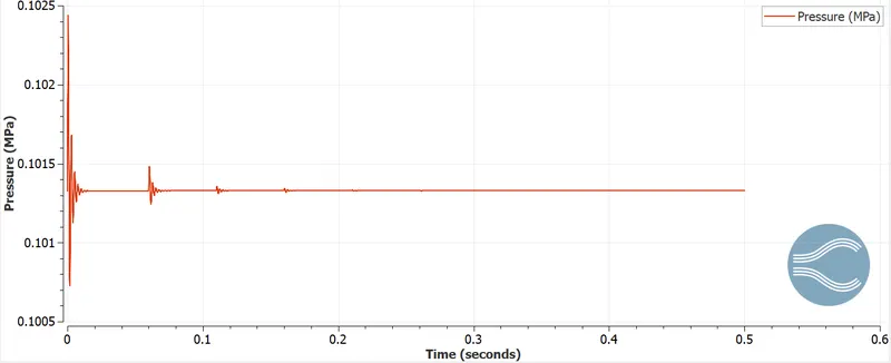
The difference between inlet and outlet pressure is measured in terms of time interval. The fluctuation of pressure is high at beginning and touches 102.4kPa and becomes steady at 101.3kPa. Initial pressure is high because of convective heat transfer from air. With increase in interval small fluctuation are to be seen due to super cycle interval at the solid and become stable gradually.
Mean temperature:
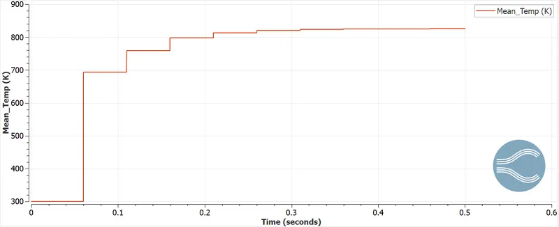
The mean temp is fluctuating with respect to time. After 0.1s the temperature shoots to 750k because of convective heat transfer at a faster rate. The solid horizontal line indicates the time taken for the solid domain to heat up.
Velocity:
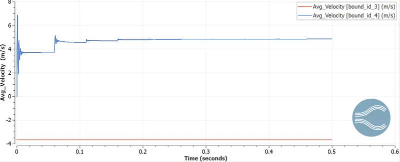
The velocity fluctuation is also a function of pressure change. Similar to pressure fluctuation, velocity is high initially as 6.5m/s and then with super cycling stages, the fluctuation reduces and become stable.
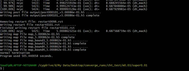
Computation time:
Contours
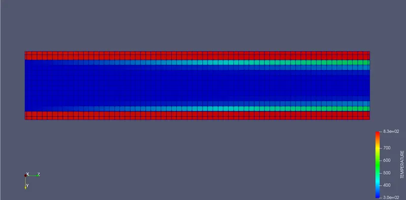
Temperature
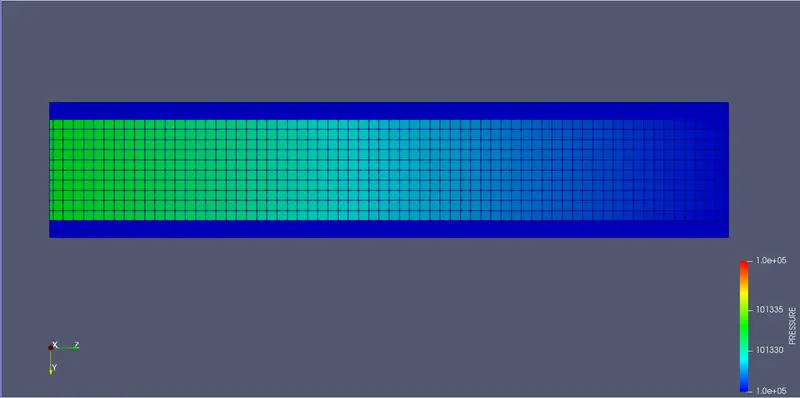
Pressure
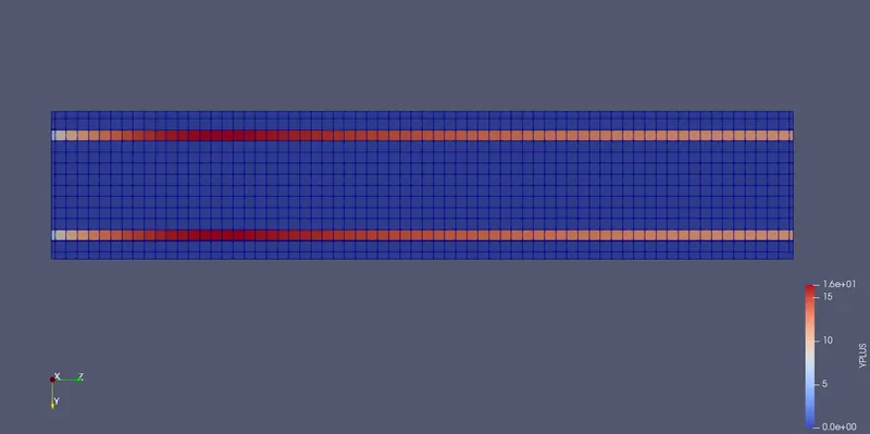
Y+ plot
cell count
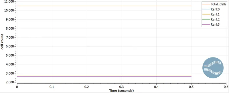
Total cell count is achieved about 10000 cells and for processor 0, 1, 2 and 3 have in between 2000-3000 cells.
Animation
Temperature
pressure
y+
Super cycle interval: 0.02s
Mesh
Region ID
Graphical analysis
Pressure:
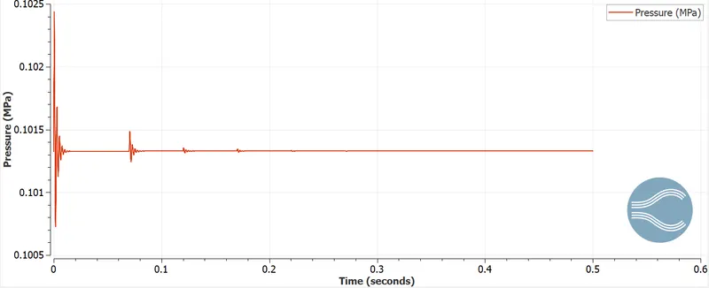
The difference between inlet and outlet pressure is measured in terms of time interval. The fluctuation of pressure is high at beginning and touches 102.4kPa and becomes steady at 101.3kPa. Initial pressure is high because of convective heat transfer from air. With increase in interval small fluctuation are to be seen due to super cycle interval at the solid and become stable gradually.
Mean temperature:
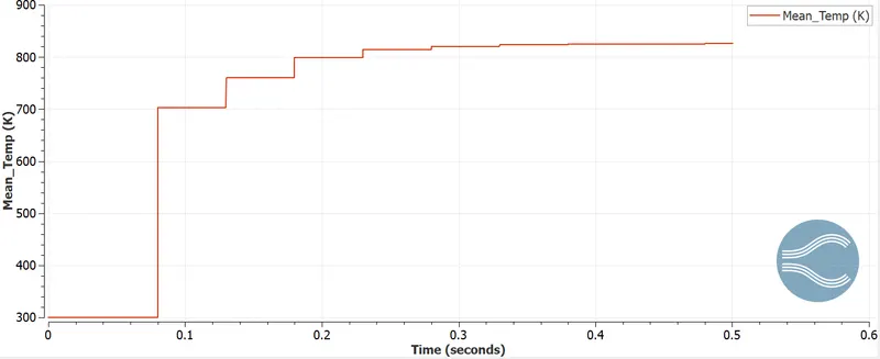
The mean temp is fluctuating with respect to time. After 0.1s the temperature shoots to 750k because of convective heat transfer at a faster rate. The solid horizontal line indicates the time taken for the solid domain to heat up.
Velocity:
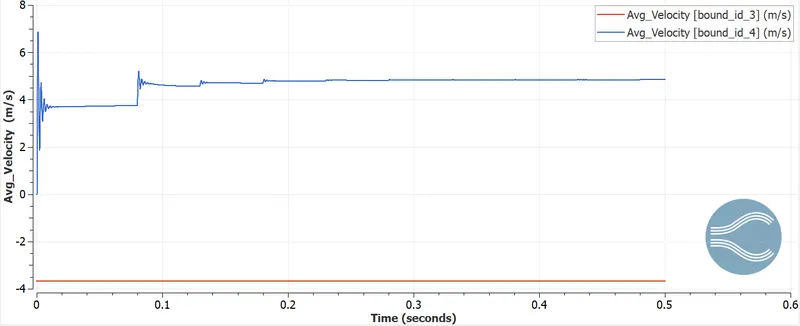
The velocity fluctuation is also a function of pressure change. Similar to pressure fluctuation, velocity is high initially as 6.5m/s and then with super cycling stages, the fluctuation reduces and become stable.
Computation time:
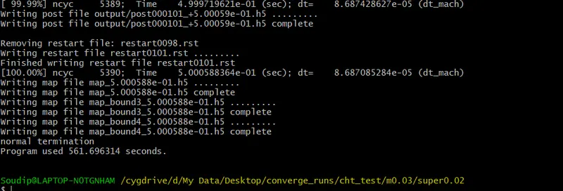
Contours
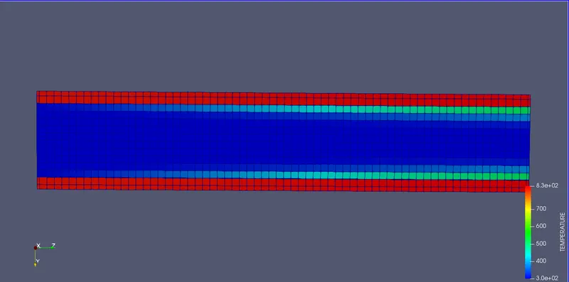
Temperature
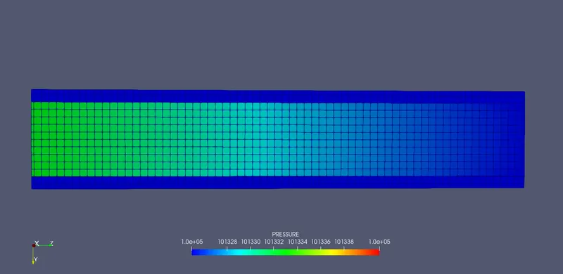
Pressure
Y+ plot
cell count
Total cell count is achieved about 5000 cells and for processor 0, 1, 2 and 3 have in between 1000-1500 cells.
Animation
Temperature
pressure
y+
Super cycle interval: 0.03s
Mesh
Region ID
Graphical analysis
Pressure:
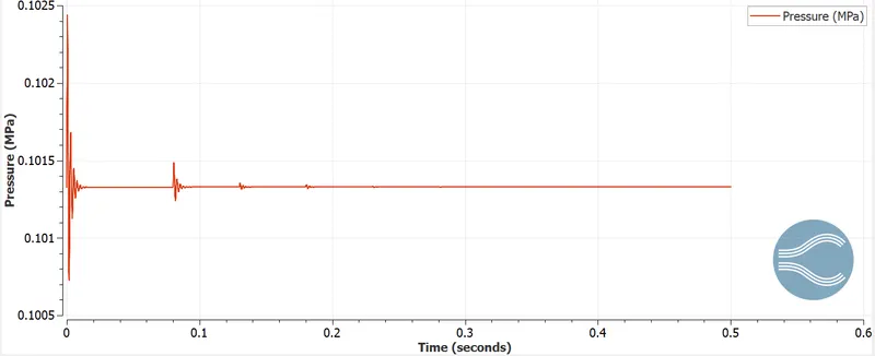
The difference between inlet and outlet pressure is measured in terms of time interval. The fluctuation of pressure is high at beginning and touches 102.4kPa and becomes steady at 101.3kPa. Initial pressure is high because of convective heat transfer from air. With increase in interval small fluctuation are to be seen due to super cycle interval at the solid and become stable gradually.
Mean temperature:
The mean temp is fluctuating with respect to time. After 0.1s the temperature shoots to 700k because of convective heat transfer at a faster rate. The solid horizontal line indicates the time taken for the solid domain to heat up.
Velocity:
The velocity fluctuation is also a function of pressure change. Similar to pressure fluctuation, velocity is high initially as 6.5m/s and then with super cycling stages, the fluctuation reduces and become stable.
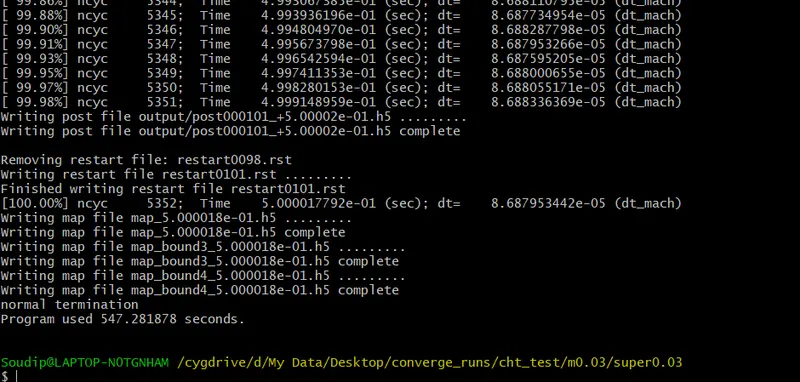
Computation time:
Contours
Temperature
Pressure
Y+ plot
cell count
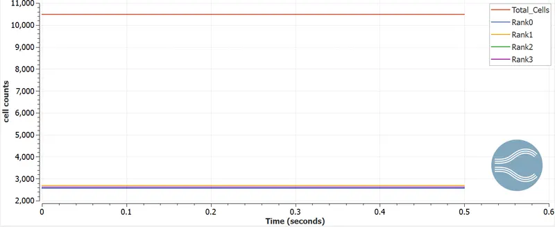
Total cell count is achieved about 10000 cells and for processor 0, 1, 2 and 3 have in between 2000-3000 cells.
Animation
Temperature
pressure
y+
Case 3
Refined grid 0.002m
Super cycle interval: 0.01s
Mesh
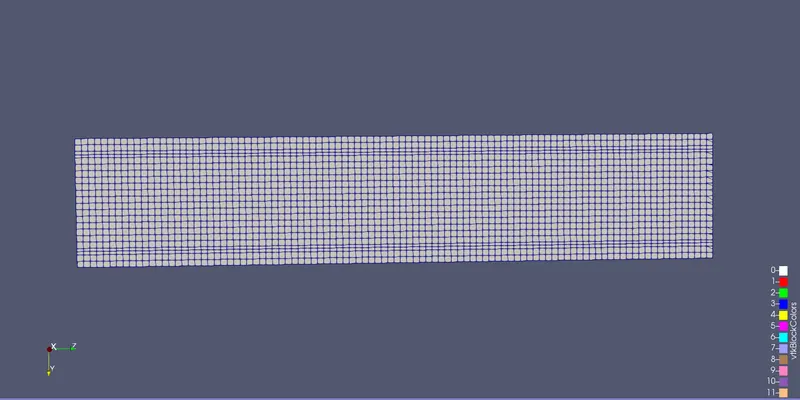
Graphical analysis
Pressure:
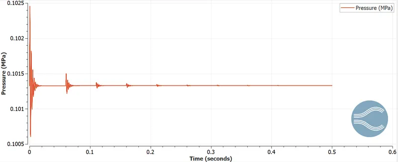
The difference between inlet and outlet pressure is measured in terms of time interval. The fluctuation of pressure is high at beginning and touches 102.4kPa and becomes steady at 101.3kPa. Initial pressure is high because of convective heat transfer from air. With increase in interval small fluctuation are to be seen due to super cycle interval at the solid and become stable gradually.
Mean temperature:
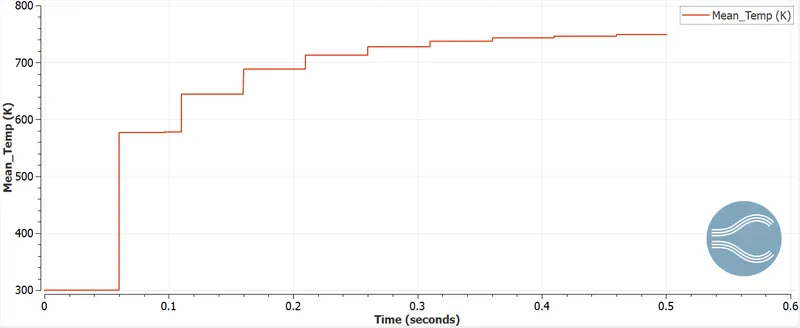
The mean temp is fluctuating with respect to time. After 0.1s the temperature shoots to 750k because of convective heat transfer at a faster rate. The solid horizontal line indicates the time taken for the solid domain to heat up.
Velocity:
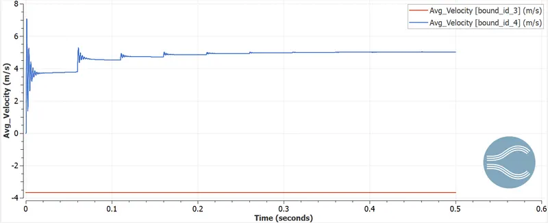
The velocity fluctuation is also a function of pressure change. Similar to pressure fluctuation, velocity is high initially as 6.5m/s and then with super cycling stages, the fluctuation reduces and become stable.
Computation time:
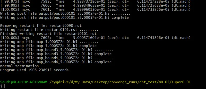
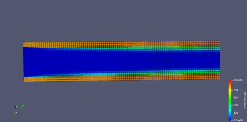
Contours
Temperature
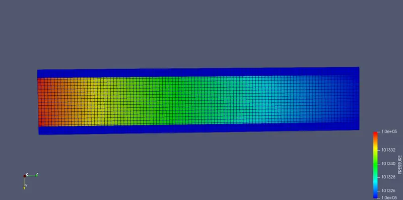
Pressure
Y+ plot
cell count
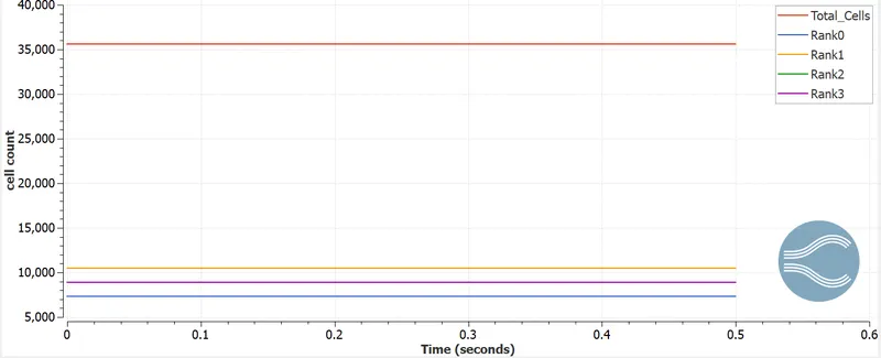
Total cell count is achieved about 38000 cells and for processor 0, 1, 2 and 3 have in between 10000-7500 cells.
Animation
Temperature
pressure
y+
Super cycle interval: 0.02s
Mesh
Region ID
Graphical analysis
Pressure:
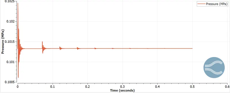
The difference between inlet and outlet pressure is measured in terms of time interval. The fluctuation of pressure is high at beginning and touches 102.4kPa and becomes steady at 101.3kPa. Initial pressure is high because of convective heat transfer from air. With increase in interval small fluctuation are to be seen due to super cycle interval at the solid and become stable gradually.
Mean temperature:
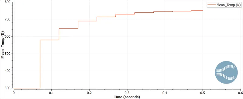
The mean temp is fluctuating with respect to time. After 0.1s the temperature shoots to 750k because of convective heat transfer at a faster rate. The solid horizontal line indicates the time taken for the solid domain to heat up.
Velocity:
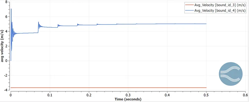
The velocity fluctuation is also a function of pressure change. Similar to pressure fluctuation, velocity is high initially as 7.5m/s and then with super cycling stages, the fluctuation reduces and become stable.
Computation time:
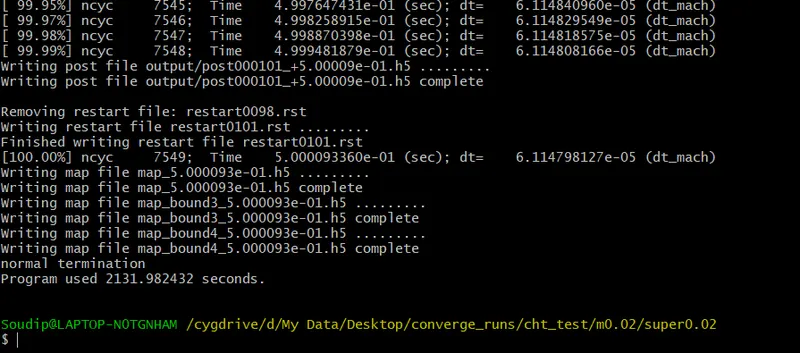
Contours
Temperature
Pressure
Y+ plot
cell count
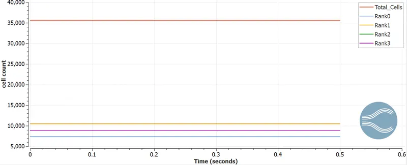
Total cell count is achieved about 35000 cells and for processor 0, 1, 2 and 3 have in between 10000-8000 cells.
Animation
Temperature
pressure
y+
Super cycle interval: 0.03s
Mesh
Region ID
Graphical analysis
Pressure:
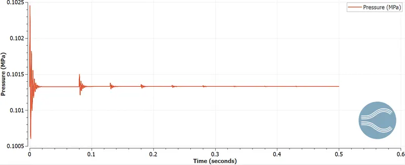
The difference between inlet and outlet pressure is measured in terms of time interval. The fluctuation of pressure is high at beginning and touches 102.4kPa and becomes steady at 101.3kPa. Initial pressure is high because of convective heat transfer from air. With increase in interval small fluctuation are to be seen due to super cycle interval at the solid and become stable gradually.
Mean temperature:
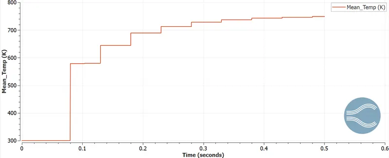
The mean temp is fluctuating with respect to time. After 0.1s the temperature shoots to 750k because of convective heat transfer at a faster rate. The solid horizontal line indicates the time taken for the solid domain to heat up.
Velocity:
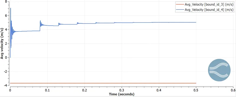
The velocity fluctuation is also a function of pressure change. Similar to pressure fluctuation, velocity is high initially as 6.5m/s and then with super cycling stages, the fluctuation reduces and become stable.
Computation time:
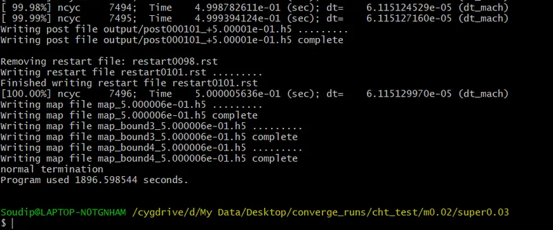
Contours
Temperature
Pressure
Y+ plot
cell count
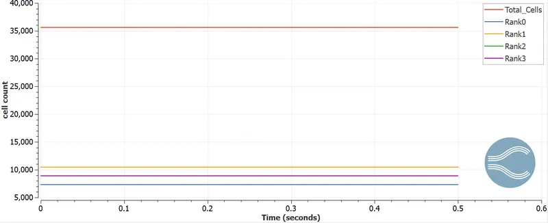
Total cell count is achieved about 35000 cells and for processor 0, 1, 2 and 3 have in between 10000-5000 cells.
Animation
Temperature
pressure
y+
Comparison of mean temperature at the solid interface for grid scale 3
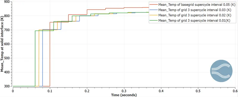
On comparing with the base grid super cycle, it is seen that the maximum temperature reached is 850k. But for the refined scale of 3, the maximum temperature is less compared to base grid and reaches maximum up to 810k. On refining the grid, the super cycle time for heating the solid domain speeds up and within less than 0.1s for super cycle interval of 0.003s increases to 700k. The similar pattern is noted for other super cycle interval, but important to see that with decreasing the super cycle interval, the conjugate heat transfer process fasten up with more accuracy and efficiently.
Comparison of mean temperature at the solid interface for grid scale 2
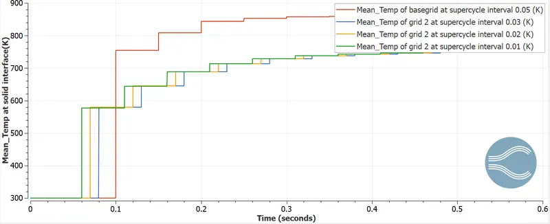
The same noted phenomenon can be seen as in grid scale 3. Over here in this case there is a drastic reduction of time and temperature plot. The maximum temperature is about 750k, which is even less compared to grid size 3. The efficiency in capturing the solid temperature change is more accurate. One interesting point to be noted that the difference between the super cycle interval for the refined and base line is more and with increasing in time interval it reaches a stable point.
Comparison of mean temperature at the fluid interface for grid scale 3
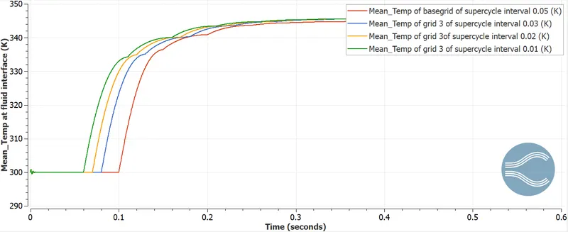
The fluid interface heat interaction takes place faster than solid due to less heat capacity. Also the maximum temperature achieved is less compared to that of the solid region and reaches maximum of 345k. Also with different super cycle interval, the temperature quickly rises even before the time scale is reached for the base line grid. With super cycling the speed for heat exchange and also with refining the grid gets more accurate and finer results.
Comparison of mean temperature at the fluid interface for grid scale 2
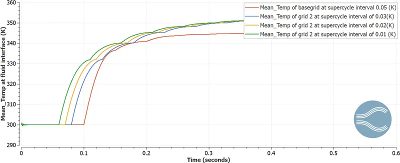
The mean temperature distribution for the base grid and refined scale have a large temperature difference. With finer refinement and different super cycle interval, the temperature scale reaches faster and the physics of heat exchange is captured in a more detailed way.
y+ data:
y+ is a non dimensional scale that is normalised at the wall. Since each turbulence model simulates boundary conditions, so the value of y+ is very important to predict the flow field of boundary layer. Maximum value of y+ obtained for different mesh size according to cases
grid 4mm, y+=16mm
grid 3mm, y+=16mm
grid 2mm, y+=16mm
the y+ value lies in between 5 to 30, so it lies within buffer region.
Conclusions:
- From the refined grid independency test, it is found that conjugate heat transfer process between the solid and fluid region is accurately predicted with less time.
- Super cycle modelling is performed to achieve more accurate and fast results. Super cycle model speeds up the computation process to achieve stability quicker.
- On increasing the grid size, the computational cells increase and also time. But with increase in super cycling time interval, it increases efficiency of the process.
- The interface of solid and fluid domain is captured accurately by super cycle model. With high Reynolds no, value of air passing through pipe enables to capture the velocity, pressure and temperature at the outlet section.