Week 7 - Auto ignition using Cantera

Theory:

Auto ignition occurs when a mixture of gases or vapours ignites spontaneously in absence of any external sources such as flame or spark. The temperature at which the auto ignition occurs is called auto ignition temperature. It is the lowest temperature in a system where the rate of heat evolved from gases or vapours increases beyond the rate of heat loss to the surrounding, resulting in ignition. The auto ignition is not an intrinsic property of gases or vapours and is affected by temperature, vessel shape, volume, reactant concentration and reaction rate.

A cantera reactor network represents the simplest form of a chemically reacting system. It corresponds to an extensive thermodynamic volume V, in which all the state variables are homogeneously distributed. Transient state change due to chemical reactions are possible, however thermodynamic equilibrium is assumed to be present through out the reaction at all time.

The ReactorNet () object is used to model reactor clss. The advance(time) function is used to advance the reactor state to a specific time. This thermodynamic state of the reactor can then be extracted at each time step to study the transient behaviour of the reactor.

Governing equations:

Mass conservation

`(dm)/dt=∑(m_(i)) ̇-∑(m_o )+ m_wall`

Species conservation

`m_k=V_w W_k+m_wall`

Energy conservation

`U=m∑Y_k u_k (T)`

Objective:

PART I

Use the same reactor network code as shown in the video to simulate the Auto Ignition Time for Methane under the following conditions, (simulation time = 10 secs)

• Plot the variation of Auto Ignition time of Methane with a constant temperature of 1250K and pressure varying from 1 to 5 atm.
• Plot the variation of Auto Ignition time of Methane with a constant pressure of 5 atm and temperature varying from 950K to 1450K.

NOTE:

Auto Ignition time is the time when the temperature of the reactor is Initial Temperature plus 400K.

PART II

Further, observe and print the rate of change of molar concentrations of the given elements "H2O, O2, OH" with respect to the time, (simulation time = 10 secs)

Explain the behavior of the graph for 2 cases,

• When Temperature is 1000K and pressure 5 bar
• When Temperature is 500K and pressure 5 bar

PYTHON CODE FOR AUTO IGNITION TEMPERATURE AT VARIABLE PRESSURE

# import libraries
import sys
import numpy as np
import cantera as ct
import matplotlib.pyplot as plt

# define the pressure range
pressure=np.linspace(1,5,5)
#initial temperature
T=1250
# species dictionary
species_dic={'CH4':1,'O2':2,'N2':7.52}
# total time for simulation
simulation_time=10
step_time=1e-3
# calculating the no of time steps
time_steps=int(simulation_time/step_time)

#array for auto ignition delay
Auto_ig_time=[]
# loop for pressure variation

for i in pressure:
	# create gas object

	gas=ct.Solution('gri30.xml')
	# convert pressure from atm to Pa
	p=i*101325
	# provide initial condition to gaas object

	gas.TPX=T,p,species_dic
	# reactor instances of solution class
	r=ct.IdealGasReactor(gas)

	# creating reactor network
	sim=ct.ReactorNet([r])
	# initial time
	time =0
	# preparing solution array for each state
	states=ct.SolutionArray(gas,extra=['time_ms'])

	loop_counter=0

	#time loop(time integration for states)

	for n in range (time_steps):
		time+=step_time
		# advancing time

		sim.advance(time)
		states.append(r.thermo.state,time_ms=time/step_time)
		#loop to compute ignition delay

		if((states.T[n]>=(T+400))and loop_counter==0):
			Auto_ig_time.append(states.time_ms[n])
			loop_counter=1


	plt.figure(1)
	plt.plot(states.time_ms,states.T)
	plt.legend(['pressure='+str(int(i))+'atm' for i in pressure])

plt.figure(1)
plt.grid('on')
plt.xlabel('time in milli second')
plt.ylabel('Auto ignition in temperature in K')
plt.title('variation in auto ignition temperature for variable initial pressure')

plt.figure(2)
plt.grid('on')
plt.plot(pressure,Auto_ig_time,'-o',color='blue')
plt.xlabel('pressure in atm')
plt.ylabel('Auto ignition delay in milli sec')
plt.title('variation in auto ignition temperature for variable initial pressure')
plt.show()

Graphical plot

fig 1

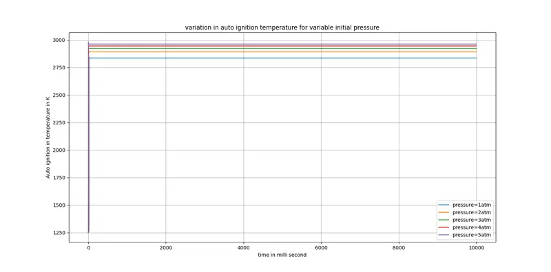
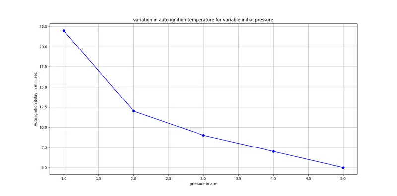
fig 2

PYTHON CODE FOR AUTO IGNITION TEMPERATURE AT VARIABLE INITIAL TEMPERATURE

# importing libraries
import sys
import numpy as np
import cantera as ct
import matplotlib.pyplot as plt

# initial temperature in K
temp=np.linspace(950,1450,5)
# initial pressure in Pa
p=5*101325
# species dictionary
species_dic={'CH4':1,'O2':2,'N2':7.52}
# total time for simulation
simulation_time=10

step_time=1e-3
# calculating the no of time steps
time_steps=int(simulation_time/step_time)

#array for auto ignition delay
Auto_ig_time=[]
# loop for pressure variation

for T in temp:
	# create gas object

	gas=ct.Solution('gri30.xml')
	
	# provide initial condition to gaas object

	gas.TPX=T,p,species_dic
	# reactor instances of solution class
	r=ct.IdealGasReactor(gas)

	# creating reactor network
	sim=ct.ReactorNet([r])
	# initial time
	time =0
	# preparing solution array for each state
	states=ct.SolutionArray(gas,extra=['time_ms'])

	loop_counter=0

	#time loop(time integration for states)

	for n in range (time_steps):
		time+=step_time
		# advancing time

		sim.advance(time)
		states.append(r.thermo.state,time_ms=time/step_time)
		#loop to compute ignition delay

		if((states.T[n]>=(T+400))and loop_counter==0):
			Auto_ig_time.append(states.time_ms[n])
			loop_counter=1

	plt.figure(1)
	plt.plot(states.time_ms,states.T)
	plt.legend(['temperature='+str(int(T))+'K' for T in temp])

plt.figure(1)
plt.grid('on')
plt.xlabel('time in milli second')
plt.ylabel('Auto ignition in temperature in K')
plt.title('variation in auto ignition temperature for variable temperature')

plt.figure(4)
plt.grid('on')
plt.plot(temp,Auto_ig_time,'-o',color='red')
plt.xlabel('Ignition temperature in K')
plt.ylabel('Auto ignition delay in milli sec')
plt.title('variation in auto ignition delay for variable temperature')
plt.show()

Graphical plot

fig 3

 

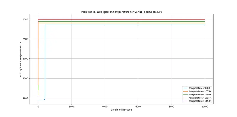
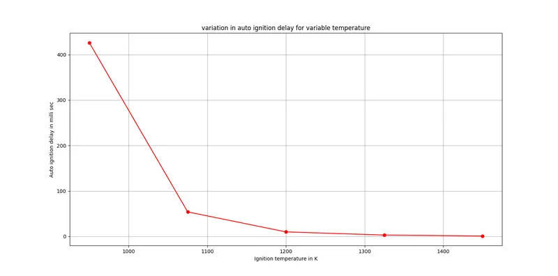
fig 4

PYTHON CODE FOR  AT VARIABLE INITIAL TEMPERATURE FOR MOLAR SPECIES CONCENTRATION

# importing libraries
import sys
import numpy as np
import cantera as ct
import matplotlib.pyplot as plt

# initial temperature in K
temp=[500,1000]
# initial pressure in Pa
p=5*101325
# species dictionary
species_dic={'CH4':1,'O2':2,'N2':7.52}
# total time for simulation
simulation_time=10

step_time=1e-3
# calculating the no of time steps
time_steps=int(simulation_time/step_time)

#array for auto ignition delay
Auto_ig_time=[]
# loop for pressure variation

for T in temp:
	# create gas object

	gas=ct.Solution('gri30.xml')
	
	# provide initial condition to gas object

	gas.TPX=T,p,species_dic
	# reactor instances of solution class
	r=ct.IdealGasReactor(gas)

	# creating reactor network
	sim=ct.ReactorNet([r])
	# initial time
	time =0
	# preparing solution array for each state
	states=ct.SolutionArray(gas,extra=['time_ms'])

	loop_counter=0
	#time loop(time integration for states)

	for n in range (time_steps):
		time+=step_time
		# advancing time

		sim.advance(time)
		states.append(r.thermo.state,time_ms=time/step_time)
		#loop to compute ignition delay

		if((states.T[n]>=(T+400))and loop_counter==0):
			Auto_ig_time.append(states.time_ms[n])
			loop_counter=1

	plt.figure(T)

	plt.subplot(1,3,1)
	plt.plot(states.time_ms,states.X[:,gas.species_index('H2O')],color='blue')
	plt.xlabel('time in milli-second')
	plt.ylabel('Mole fraction of species')
	plt.legend(['H2O'])

	plt.subplot(1,3,2)
	plt.plot(states.time_ms,states.X[:,gas.species_index('OH')],color='red')
	plt.xlabel('time in milli-second')
	plt.ylabel('Mole fraction of species')
	plt.legend(['OH'])

	plt.subplot(1,3,3)
	plt.plot(states.time_ms,states.X[:,gas.species_index('O2')],color='green')
	plt.xlabel('time in milli-second')
	plt.ylabel('Mole fraction of species')
	plt.legend(['O2'])
	plt.suptitle('Mole fraction of species for temperature='+str(int(T))+'K' )	
plt.show()

Graphical plot

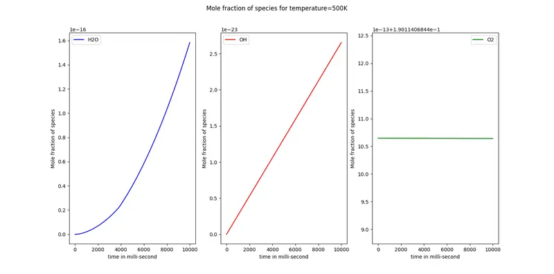
AT T=500K

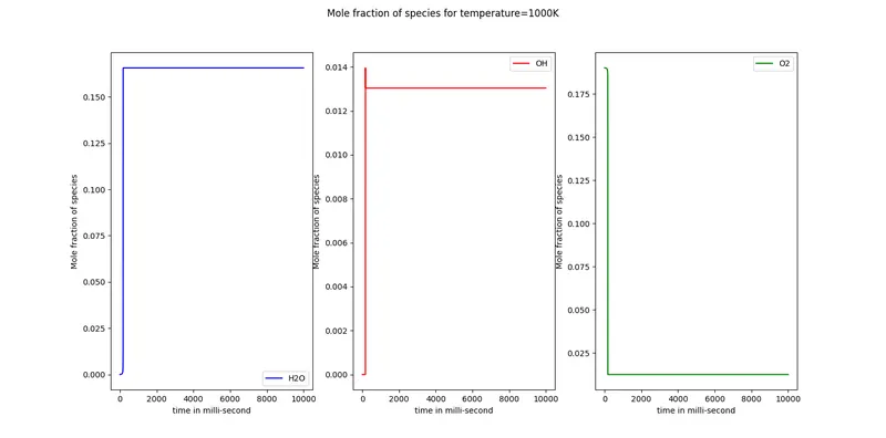
AT T=1000K

At T=500K, it is observed that there is no variation in the mole fraction of O2, whereas in element H2O and OH it varies slightly. This happens due to the bond structure of molecules. Those are single bond molecules and apparently require less temperature to break or react. Whereas O2 has double bond and requires more temperature to break the bond.

For the plot of initial temperature of T=1000K, the sudden change (spike/drop) in concentration represents the stage of auto ignition with same ignition delay.

• The H2O mole fraction is increased and then stabled down with simulation time. This happens due to H2O is the product in methane fuel consumption.
• The OH mole fraction is also similar to H2O it increases and then becomes stable. It is also a product of methane combustion.
• The O2 mole fraction decreases suddenly and maintains stability. The O2 is on the reactant side of the methane combustion and gets consumed on further reactions.

Conclusions:

• As initial pressure increases, ignition delay increases.
• With increase in initial pressure, initial temperature also increases slightly.
• Increment in initial temperature results in lowering in ignition delay.
• For high initial temperature, the ignition temperature is also high and vice-versa.
• Using 500K as initial temperature is not as better as 1000K because ignition temperature of methane is more than 810K.