Prandtl Meyer Shock problem analysis using AMR technique in CONVERGE CFD
Abstract:
In this project, a 2D supersonic flow simulation is done to capture the Prandtl-Meyer shock wave propagation through the sharp corners. Adaptive mesh refinement technique is done to capture the variation of velocity, shock wave, Mach no, temperature and pressure distribution along the zones of disturbances. For turbulent modelling RNG k-epsilon model is chosen. With different sub grid scaling at subsonic and supersonic speed, the flow distribution pattern is analyzed.
Aim:
To study Prandlt Mayer shock wave problem through a 2D supersonic flow.
Objective:
1. Shock flow boundary conditions
Do a literature search on what BC's are typically used for shock flow problems
2. What is a shock wave?
In your own words, describe the physics behind shock waves
3. Effect of SGS parameter on shock location
In the Prandtl Meyer shock problem, look at the effect of SGS temperature value on cell count and the shock location
Introduction:
In physics, a shock wave (also spelled shockwave), or shock, is a type of propagating disturbance that moves faster than the local speed of sound in the medium. Like an ordinary wave, a shock wave carries energy and can propagate through a medium but is characterized by an abrupt, nearly discontinuous, change in pressure, temperature, and density of the medium.
For the purpose of comparison, in supersonic flows, additional increased expansion may be achieved through an expansion fan, also known as a Prandtl–Meyer expansion fan. The accompanying expansion wave may approach and eventually collide and recombine with the shock wave, creating a process of destructive interference. The sonic boom associated with the passage of a supersonic aircraft is a type of sound wave produced by constructive interference. Unlike solitons (another kind of nonlinear wave), the energy and speed of a shock wave alone dissipates relatively quickly with distance. When a shock wave passes through matter, energy is preserved but entropy increases. This change in the matter's properties manifests itself as a decrease in the energy which can be extracted as work, and as a drag force on supersonic objects; shock waves are strongly irreversible processes.
Shock waves can be:
Normal
At 90° (perpendicular) to the shock medium's flow direction.
Oblique
At an angle to the direction of flow.
Bow
Occurs upstream of the front (bow) of a blunt object when the upstream flow velocity exceeds Mach 1.
supersonic flows
The abruptness of change in the features of the medium, that characterize shock waves, can be viewed as a phase transition: the pressure-time diagram of a supersonic object propagating shows how the transition induced by a shock wave is analogous to a dynamic phase transition.
When an object (or disturbance) moves faster than the information can propagate into the surrounding fluid, then the fluid near the disturbance cannot react or "get out of the way" before the disturbance arrives. In a shock wave the properties of the fluid (density, pressure, temperature, flow velocity, Mach number) change almost instantaneously. Measurements of the thickness of shock waves in air have resulted in values around 200 nm (about 10−5 in),which is on the same order of magnitude as the mean free path of gas molecules. In reference to the continuum, this implies the shock wave can be treated as either a line or a plane if the flow field is two-dimensional or three-dimensional, respectively.
Shock waves are formed when a pressure front moves at supersonic speeds and pushes on the surrounding air. At the region where this occurs, sound waves travelling against the flow reach a point where they cannot travel any further upstream and the pressure progressively builds in that region; a high pressure shock wave rapidly forms.
Shock waves are not conventional sound waves; a shock wave takes the form of a very sharp change in the gas properties. Shock waves in air are heard as a loud "crack" or "snap" noise. Over longer distances, a shock wave can change from a nonlinear wave into a linear wave, degenerating into a conventional sound wave as it heats the air and loses energy. The sound wave is heard as the familiar "thud" or "thump" of a sonic boom, commonly created by the supersonic flight of aircraft.
The shock wave is one of several different ways in which a gas in a supersonic flow can be compressed. Some other methods are isentropic compressions, including Prandtl–Meyer compressions. The method of compression of a gas results in different temperatures and densities for a given pressure ratio which can be analytically calculated for a non-reacting gas. A shock wave compression results in a loss of total pressure, meaning that it is a less efficient method of compressing gases for some purposes, for instance in the intake of a scramjet. The appearance of pressure-drag on supersonic aircraft is mostly due to the effect of shock compression on the flow.
Shock capturing and detection
Computational fluid dynamics is commonly used to obtain the flow field with shock waves. Though shock waves are sharp discontinuities, in numerical solutions of fluid flow with discontinuities (shock wave, contact discontinuity or slip line), the shock wave can be smoothed out by low-order numerical method (due to numerical dissipation) or there are spurious oscillations near shock surface by high-order numerical method (due to Gibbs phenomena)
There exist some other discontinuities in fluid flow than the shock wave. The slip surface (3D) or slip line (2D) is a plane across which the tangent velocity is discontinuous, while pressure and normal velocity are continuous. Across the contact discontinuity, the pressure and velocity are continuous and the density is discontinuous. A strong expansion wave or shear layer may also contain high gradient regions which appear to be a discontinuity. Some common features of these flow structures and shock waves and the insufficient aspects of numerical and experimental tools lead to two important problems in practices:
(1) some shock waves cannot be detected or their positions are detected wrong,
(2) some flow structures which are not shock waves are wrongly detected to be shock waves.
In fact, correct capturing and detection of shock waves are important since shock waves have the following influences:
(1) causing loss of total pressure, which may be a concern related to scramjet engine performance,
(2) providing lift for wave-rider configuration, as the oblique shock wave at lower surface of the vehicle can produce high pressure to generate lift,
(3) leading to wave drag of high-speed vehicle which is harmful to vehicle performance,
(4) inducing severe pressure load and heat flux, e.g. the Type IV shock–shock interference could yield a 17 times heating increase at vehicle surface,
(5) interacting with other structures, such as boundary layers, to produce new flow structures such as flow separation, transition, etc.
A supersonic expansion fan, technically known as Prandtl–Meyer expansion fan, a two-dimensional simple wave, is a centered expansion process that occurs when a supersonic flow turns around a convex corner. The fan consists of an infinite number of Mach waves, diverging from a sharp corner. When a flow turns around a smooth and circular corner, these waves can be extended backwards to meet at a point.
Each wave in the expansion fan turns the flow gradually (in small steps). It is physically impossible for the flow to turn through a single "shock" wave because this would violate the second law of thermodynamics.
Across the expansion fan, the flow accelerates (velocity increases) and the Mach number increases, while the static pressure, temperature and density decrease. Since the process is isentropic, the stagnation properties (e.g. the total pressure and total temperature) remain constant across the fan.
Mach number (M or Ma) is a dimensionless quantity in fluid dynamics representing the ratio of flow velocity past a boundary to the local speed of sound.
`M=u/c`
where:
M is the local Mach number,
u is the local flow velocity with respect to the boundaries (either internal, such as an object immersed in the flow, or external, like a channel), and
c is the speed of sound in the medium, which in air varies with the square root of the thermodynamic temperature.
By definition, at Mach 1, the local flow velocity u is equal to the speed of sound. At Mach 0.65, u is 65% of the speed of sound (subsonic), and, at Mach 1.35, u is 35% faster than the speed of sound (supersonic). Pilots of high-altitude aerospace vehicles use flight Mach number to express a vehicle's true airspeed, but the flow field around a vehicle varies in three dimensions, with corresponding variations in local Mach number.
The local speed of sound, and hence the Mach number, depends on the temperature of the surrounding gas. The Mach number is primarily used to determine the approximation with which a flow can be treated as an incompressible flow. The medium can be a gas or a liquid. The boundary can be traveling in the medium, or it can be stationary while the medium flows along it, or they can both be moving, with different velocities: what matters is their relative velocity with respect to each other. The boundary can be the boundary of an object immersed in the medium, or of a channel such as a nozzle, diffuser or wind tunnel channeling the medium. As the Mach number is defined as the ratio of two speeds, it is a dimensionless number. If M < 0.2–0.3 and the flow is quasi-steady and isothermal, compressibility effects will be small and simplified incompressible flow equations can be used
Boundary conditions:
Boundary conditions (b.c.) are constraints necessary for the solution of a boundary value problem. A boundary value problem is a differential equation (or system of differential equations) to be solved in a domain on whose boundary a set of conditions is known. It is opposed to the “initial value problem”, in which only the conditions on one extreme of the interval are known. Boundary value problems are extremely important as they model a vast amount of phenomena and applications, from solid mechanics to heat transfer, from fluid mechanics to acoustic diffusion. They arise naturally in every problem based on a differential equation to be solved in space, while initial value problems usually refer to problems to be solved in time.
Dirichlet Boundary Condition
The Dirichlet boundary condition is a type of boundary condition named after Peter Gustav Lejeune Dirichlet
This condition specifies the value that the unknown function needs to take on along the boundary of the domain. Given, for example, the Laplace equation, the boundary value problem with the Dirichlet b.c. is written as:
`Δφ(x)=0∀x, ∈Ω`
`φ(x)=f(x)∀x,∈∂Ω`
where φ is the unknown function, x–– is the independent variable (e.g. the spatial coordinates), Ω is the function domain, ∂Ω is the boundary of the domain, and f is a given scalar function defined on ∂Ω. In the framework of numerical simulations, it is usually imposed directly in the algebraic system to be solved.
Neumann Boundary Condition
The Neumann boundary condition is a type of boundary condition, named after Carl Neumann (1832 – 1925). When imposed on an ordinary (ODE) or a partial differential equation (PDE), it specifies the values that the derivative of a solution is going to take on the boundary of the domain. Given, for example, the Laplace equation, the boundary value problem with the Neumann b.c. is written as:
`Δφ(x)=0∀,x∈Ω`
`∂φ(x)/(∂n)=f(x), ∀x∈∂Ω`
n the case of ODE (i.e. Ω⊂R1), the derivative normal to the boundary coincides with the global derivative φ′. In the rare cases in which a temporal dependency is solved through a finite element approach (instead of the more usual finite difference), this type of boundary condition is the most common. Neumann boundary condition is also called “natural” because it naturally appears in the development of the weak formulation in any finite element approach. Let’s consider the following simple equation:
`u”(x)=p(x)∀x∈R`
where u is an unknown scalar field and p is a given scalar function. This equation rules many phenomena, for instance, the thermal diffusion in 1D and the tension/compression of a beam. The finite element method consists in rewriting the equation from a differential (strong) form to an integral (weak) formulation.
The presence of the boundary term on the right-hand side highlights two properties of Neumann boundary conditions:
- homogeneous Neumann b.c. are naturally satisfied without any explicit imposition
- since Dirichlet b.c. are usually applied by modifying the right-hand term, a homogeneous Neumann condition is applied on all the boundaries where a Dirichlet b.c. is imposed.
Robin Boundary Condition
The Robin boundary condition is a type of boundary condition named after Victor Gustave Robin (1855–1897). It consists of a linear combination of the values of the field and its derivatives on the boundary. Given, for example, the Laplace equation, the boundary value problem with the Robin b.c. is written as:
`Δφ(x)=0,∀x∈Ω`
`aφ(x)+b∂φ(x)/(∂n)=f(x),∀x∈∂Ω`
Mixed Boundary Condition
It consists of applying different types of boundary conditions in different parts of the domain. It is important to notice that boundary conditions must be applied on the whole boundary: the “free” boundary is anyways subjected to a homogeneous Neumann condition. The mixed boundary condition differs from the Robin condition because the latter consists of different types of boundary conditions applied to the same region of the boundary, while the mixed condition implies different types of b.c. applied to different parts of the boundary.
Cauchy Boundary Condition
The Cauchy boundary condition is a condition on both the unknown field and its derivatives5. It differs from the Robin condition because the Cauchy condition implies the imposition of two constraints (1 Dirichlet b.c. + 1 Neumann b.c.), while the Robin condition implies only one constraint on the linear combination of the unknown function and its derivatives.
Geometrical preparation:
The supersonic flow model is imported in converge studio.
To check the dimension, go to option>> click on the geometry bounding box. To scale the geometry to proper dimension we provide a scale factor of 0.001
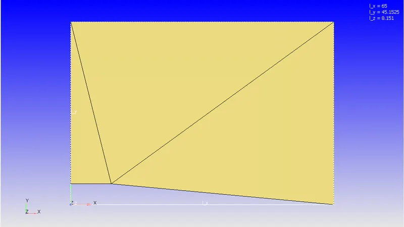
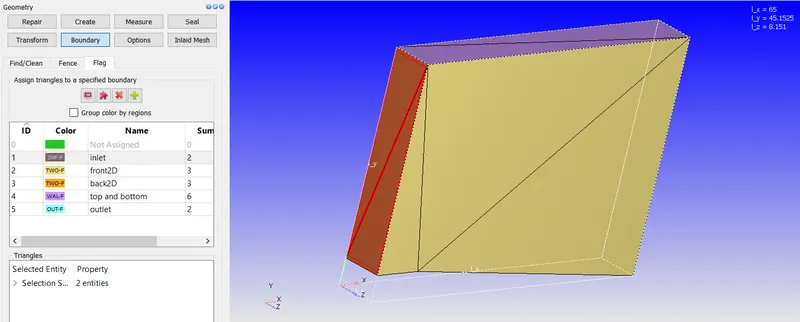
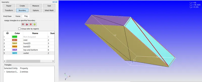
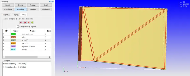
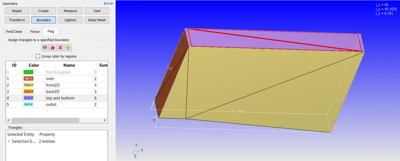
Boundary flagging: Different zones are flagged with different boundaries to with a unique ID and name given below
Inlet
Outlet
Front 2D
Back 2D
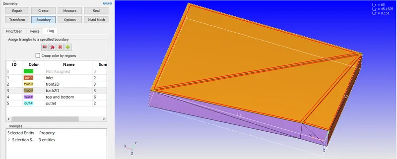
Top and bottom wall
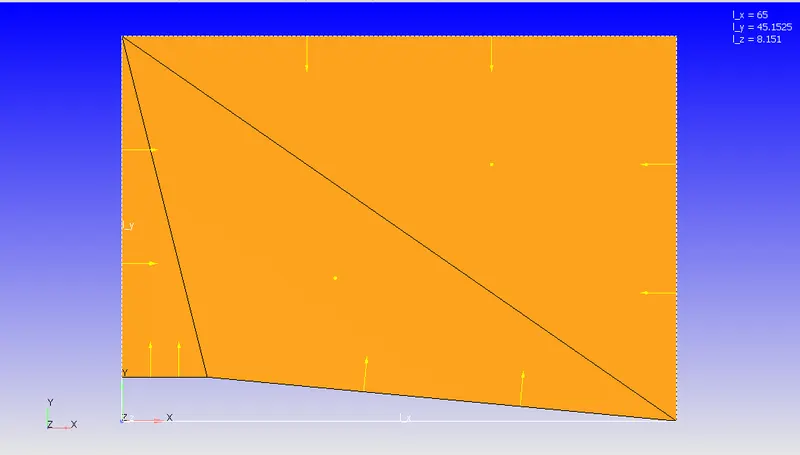
Normal orientation:
All the normal should face inward
Case setup:
Open the converge studio
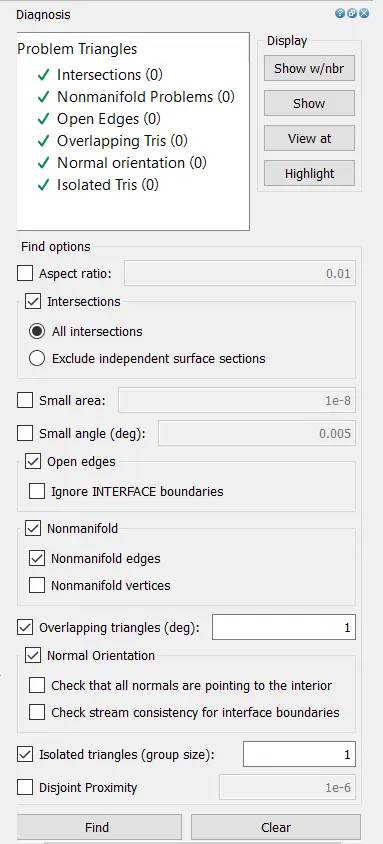
Diagnosis check up for identifying any internal error in geometry
Now we will start the case set up
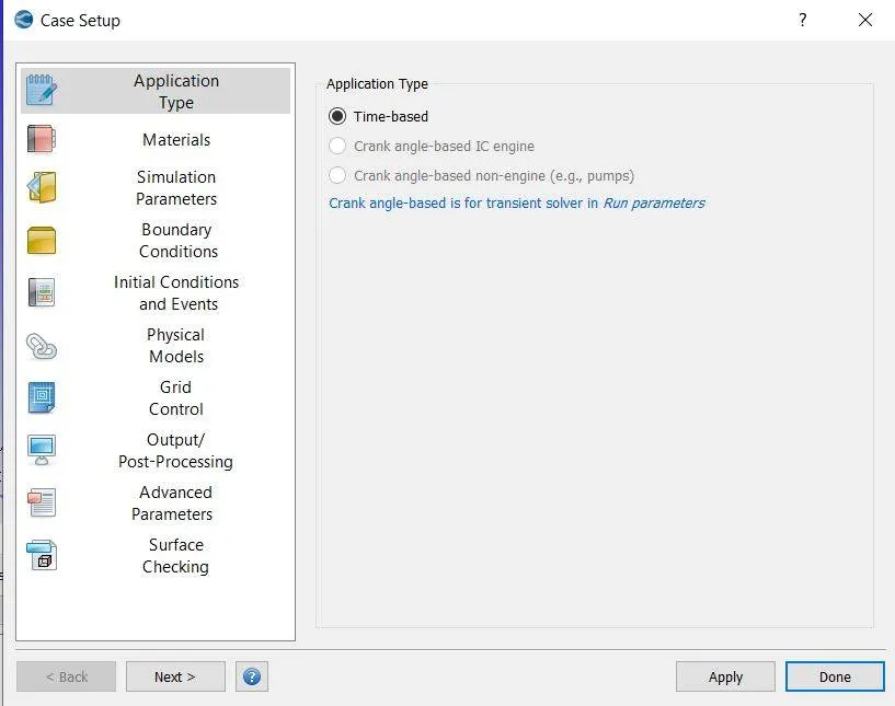
Select application option>>select time based option.
Materials
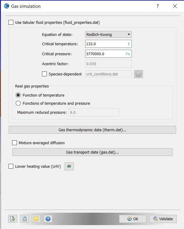
Select gas simulation> choose air as predefined mixture
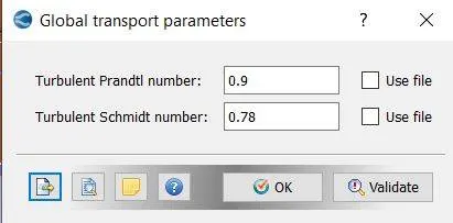
Go to global transport parameters >> select default settings>>select ok.
Solver parameter
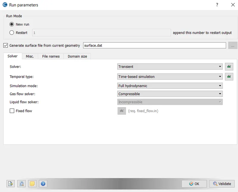
Go to simulation parameters>> select run parameters>> choose transient solver with full hydrodynamic case
solver: density based, Navier stokes equation
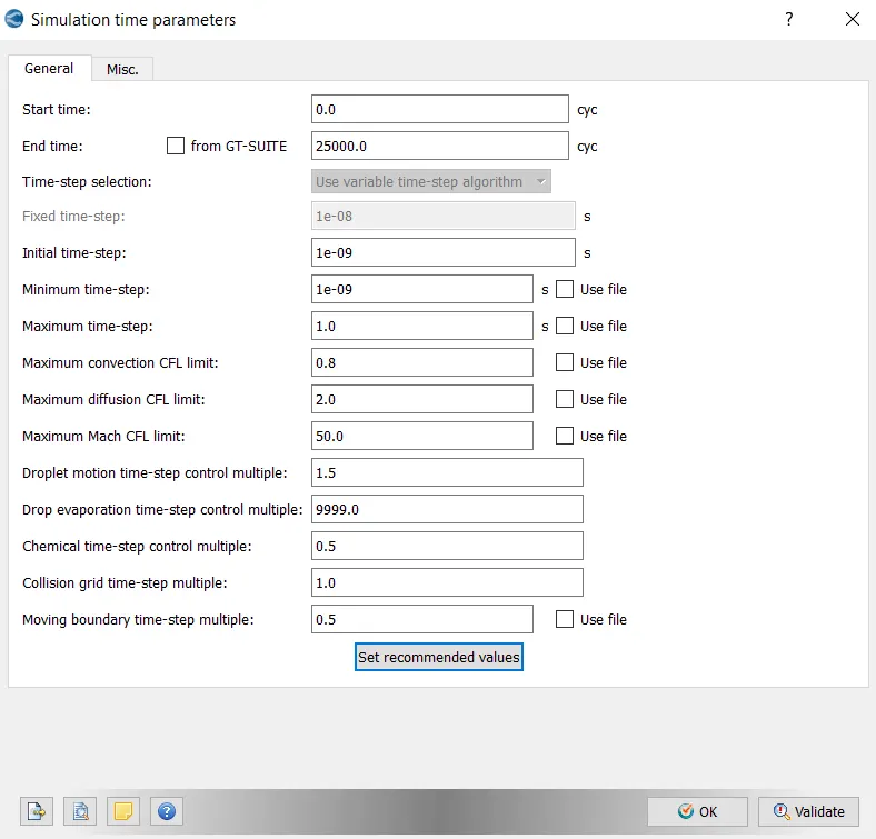
simulation time parameters
start time 0
end time 25000
initial time 1e-9
minimum time 1e-9
maximum time 1
cfl convection 0.8
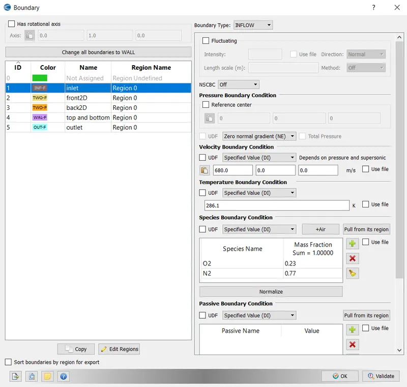
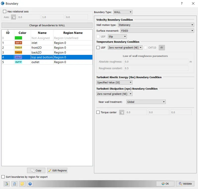
Boundary conditions:
inlet
boundary type: inflow
velocity inlet:680m/s
temperature:286.1K
pressure: zero normal gradient
species: air
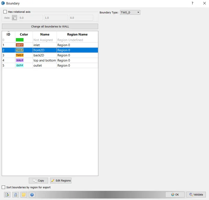
front 2D
boundary type: twoD
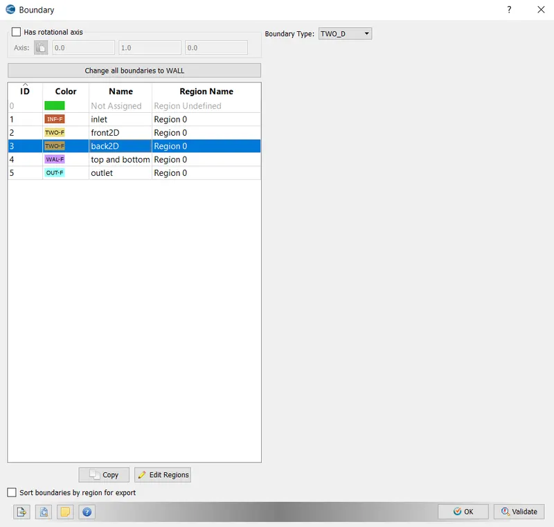
back2D
boundary type: two_D
top and bottom
boundary type: wall
wall motion: stationary
slip boundary condition
temperature: zero normal gradient
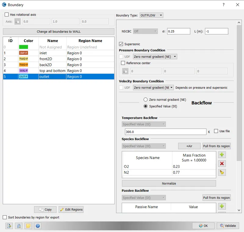
outlet
boundary type: outflow
velocity inlet:zero normal gradient
temperature:300K
pressure: zero normal gradient
species: air
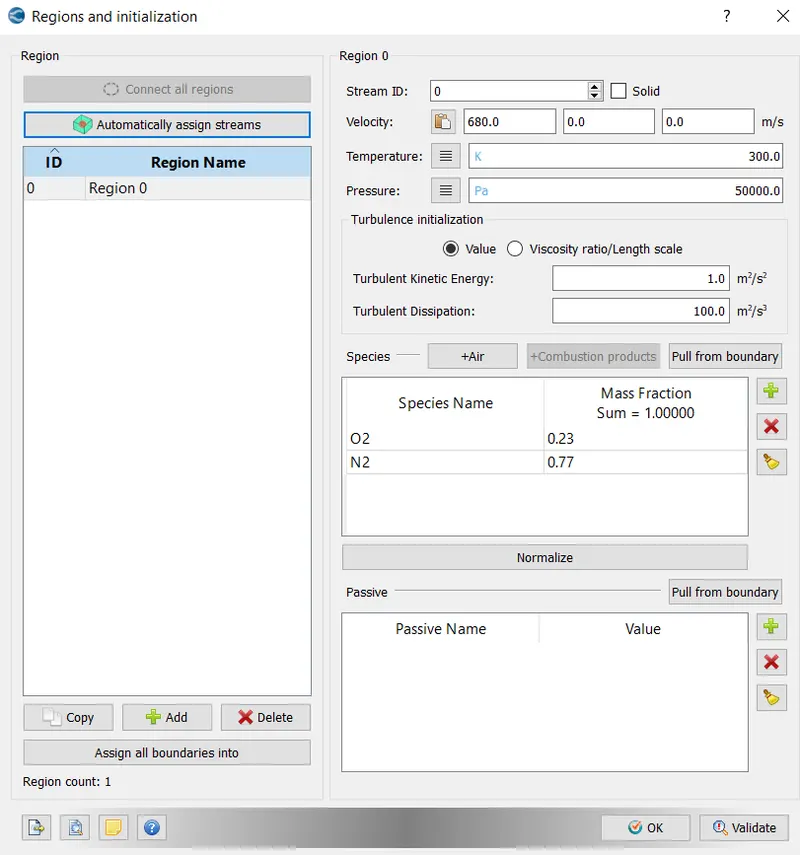
Region and initialization
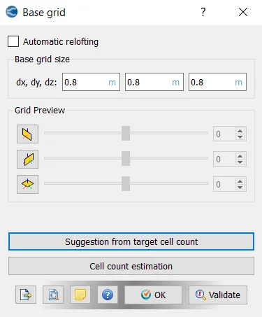
Grid control
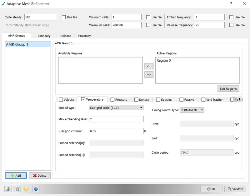
Base mesh size 0.8m
The refinement of the grid is done through embedded sizing. The formula for refinement is
Grid size=`N_(base size)/2^(embedded level) =0.8/2^2 =0.2`
check the adaptive mesh refinement
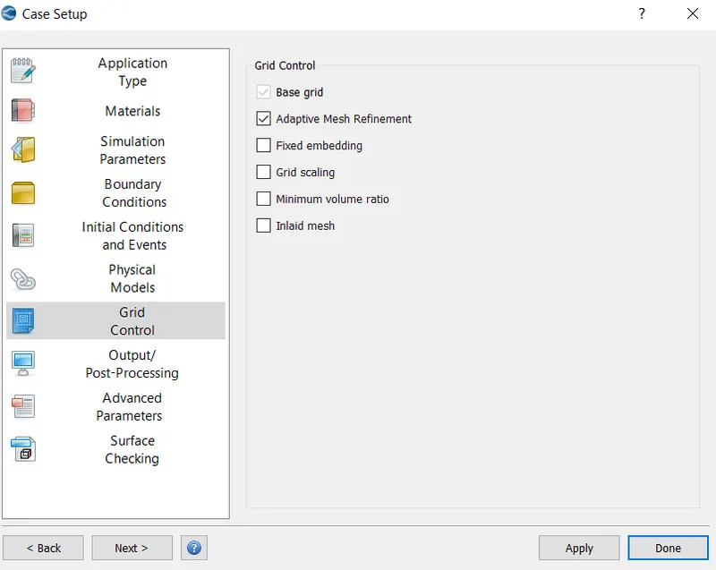
Enable adaptive mesh refinement>>go to region selection>> select region0>> choose temperature AMR settings>> embedded scale 2>> SGS value 0.05K
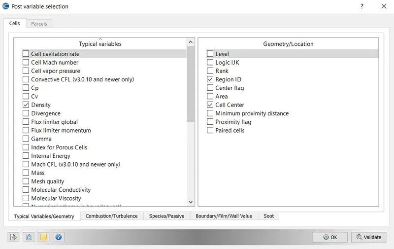
Output/post processing
Use default settings
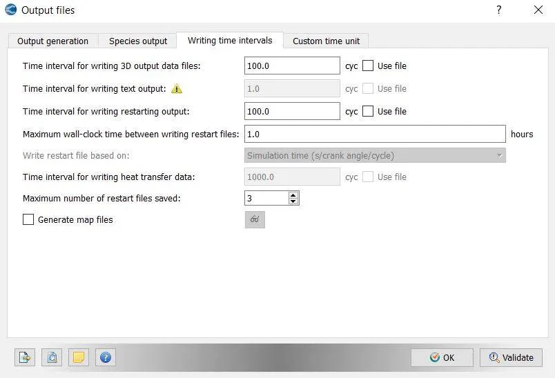
Output files
Time interval of 3D output files required is 100.0
Time required for writing restarting output file: 100
Export all the input files
go to file option>> select export>> select export input>> choose the directory>> click ok
Simulation run:
- Export all the case set up from the converge studio
- Go to Cygwin>> go to desired path or directory
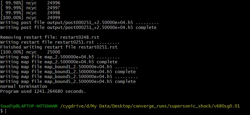
- Type the command mpiexec.exe -n 2 converge-intelmpi.exe to run the simulation.
Post processing analysis:
Case 1:
Velocity=680m/s and SGS=0.05K
Graphical analysis:
mesh:
Mass flow rate:
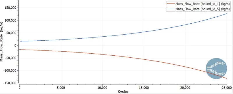
In supersonic flow with SGS 0.05k, the prandlt meyer expansion fan is visible and shock wave generation tends to diverge the mass flow at the outlet section. From the inlet section, the mass flow tends to get converged, but at the sharp turning, the pressure and velocity fluctuation starts and the mass flow quantity diverges out and reaches at 150000kg/s.
Average temperature:
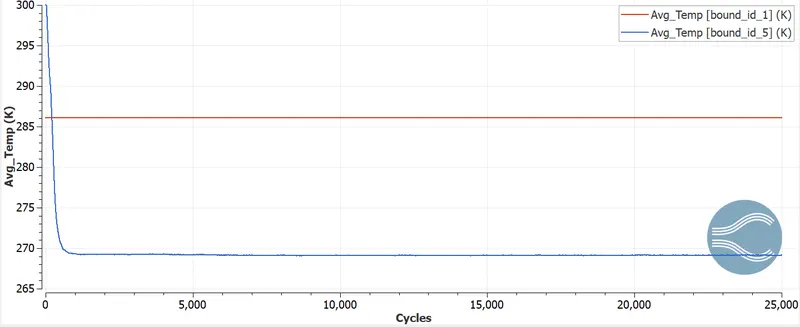
The average temperature drops after the refinement is done at the expansion region. It is seen that at the outlet section the temperature increases rapidly at the zone of sharp turn and rises to 300k, and then afterwards the temperature drops down because the temperature gets distributed at the entire surface uiformly.
Total average temperature:
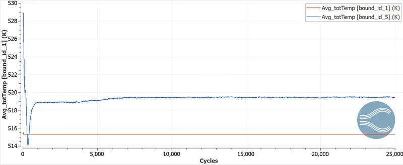
The total avg temp at the outlet is high and reaches about 519k. The outlet temp increase due to the shock wave generation and pressure fluctuation. The static pressure also increases as a function of temperature change.
Static pressure:
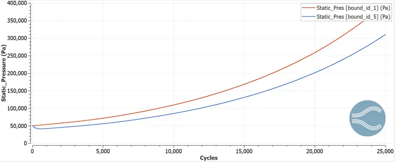
The static pressure at the inlet and outlet section is found to increase from 50000Pa to 4e5Pa. The reason for increase in pressure is due to rapid change in pressure and temperature at the sharp bent point. The shock pressure wave are lso seen to get generate and redistribute alon the entire surface.
Total pressure:
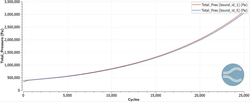
The graphical nature is same as that of the static pressure curve. Total pressure for both the inlet and outlet section also increase from 4.9e5Pa to 35e5Pa. This high rise in pressure cause the shock wave to propagate and cause high fluctuation in pressure, temperature and velocity.
Mach no:
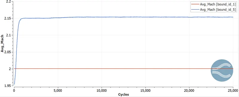
From this supersonic flow, it can be clearly seen that the outlet mach no is very high(2.15), more than that of inlet. The high mach no indicates high velocity, temperature and mass flow generation at the outlet, due to the sharp turning point causing prandlt meyer expansion wave.
Cell count:
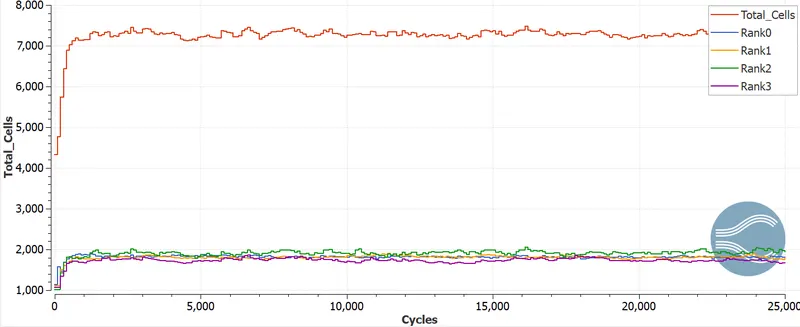
The overall cell count has reached 7500 cells. Processor 0, processor 1, processor 2 and processor 3 have cell count within the limit of 1000 to 2000 cells.
Velocity plot
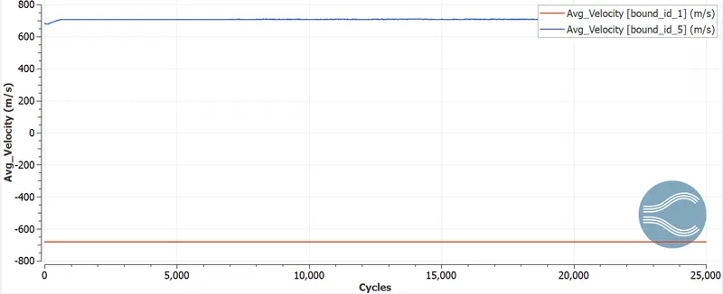
The air enters the inlet section with supersonic speed and remains constant till the sharp corner is reached. The moment the velocity passes through the bend, the outlet velocity shoots up to 741m/s, this is the cause of shock wave generation. This also proves to increase th mass flow at the outlet boundary.
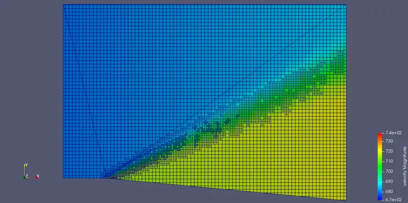
animation
Pressure plot
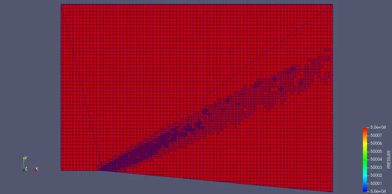
animation
Temperature plot
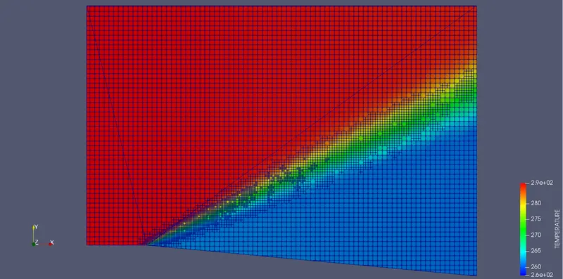
animation
Case 2:
Velocity=680m/s and SGS=0.01K
Graphical analysis:
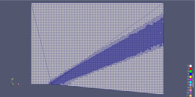
mesh
Mass flow rate:
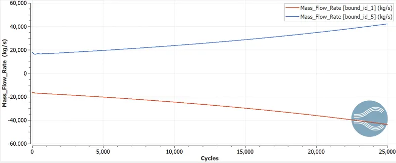
In supersonic flow with SGS 0.05k, the prandlt meyer expansion fan is visible and shock wave generation tends to diverge the mass flow at the outlet section. From the inlet section, the mass flow tends to get converged, but at the sharp turning, the pressure and velocity fluctuation starts and the mass flow quantity diverges out and reaches at 40000kg/s.
Average temperature:
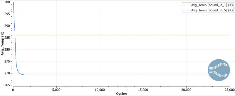
The average temperature drops after the refinement is done at the expansion region. It is seen that at the outlet section the temperature increases rapidly at the zone of sharp turn and rises to 300k, and then afterwards the temperature drops down because the temperature gets distributed at the entire surface uiformly.
Total average temperature:
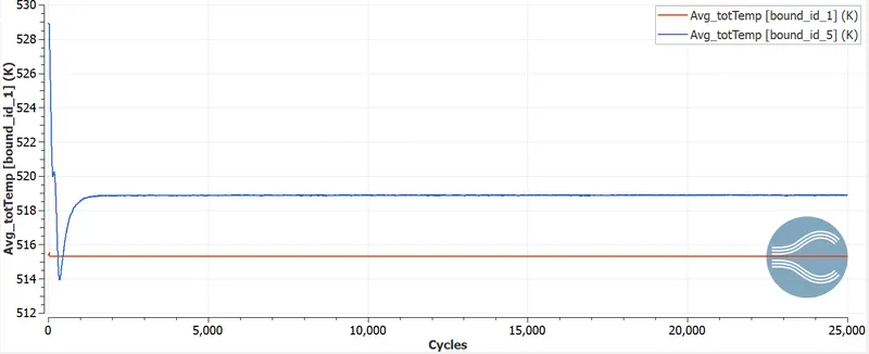
The total avg temp at the outlet is high and reaches about 529k. The outlet temp increase due to the shock wave generation and pressure fluctuation. The static pressure also increases as a function of temperature change.
Static pressure:
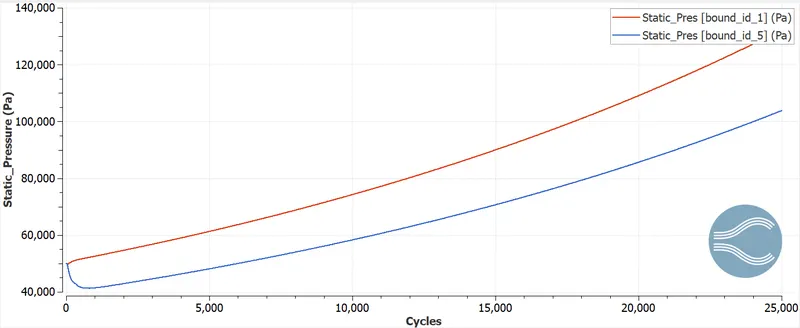
The static pressure at the inlet and outlet section is found to increase from 40000Pa to 14e5Pa. The reason for increase in pressure is due to rapid change in pressure and temperature at the sharp bent point. The shock pressure wave are lso seen to get generate and redistribute along the entire surface.
Total pressure:
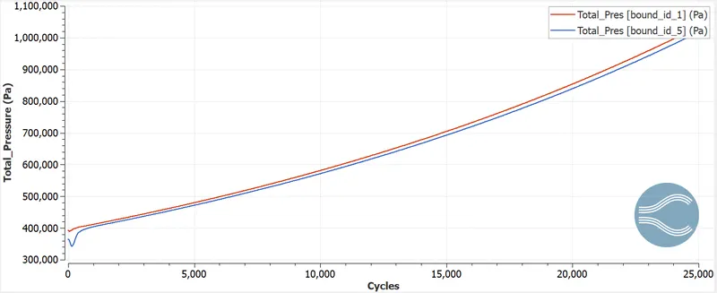
The graphical nature is same as that of the static pressure curve. Total pressure for both the inlet and outlet section also increase from 4.9e5Pa to 35e5Pa. This high rise in pressure cause the shock wave to propagate and cause high fluctuation in pressure, temperature and velocity.
Mach no:
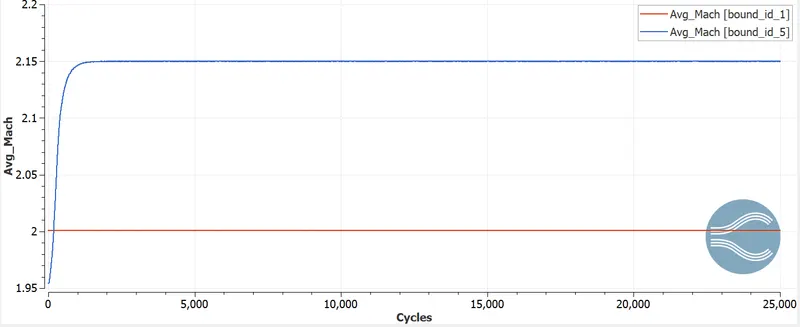
From this supersonic flow, it can be clearly seen that the outlet mach no is very high(2.15), more than that of inlet. The high mach no indicates high velocity, temperature and mass flow generation at the outlet, due to the sharp turning point causing prandlt meyer expansion wave.
Cell count:
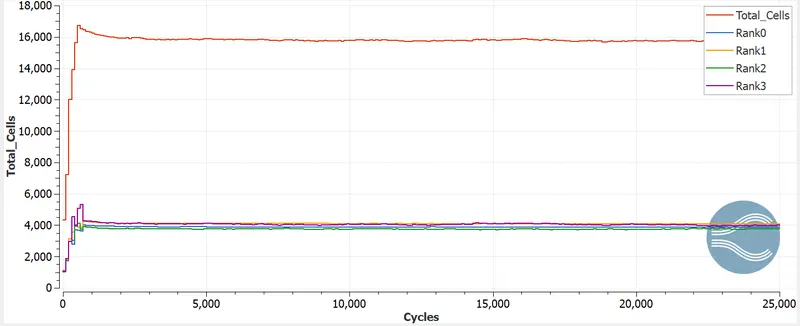
The overall cell count has reached 17000 cells. Processor 0, processor 1, processor 2 and processor 3 have cell count within the limit of 2000 to 5000 cells.
Velocity plot
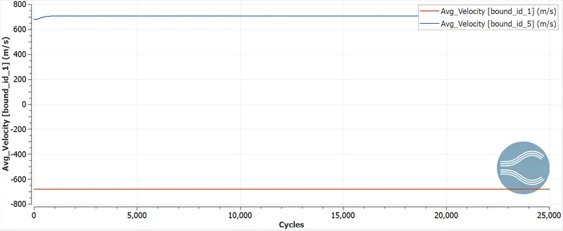
The air enters the inlet section with supersonic speed and remains constant till the sharp corner is reached. The moment the velocity passes through the bend, the outlet velocity shoots up to 741m/s, this is the cause of shock wave generation. This also proves to increase th mass flow at the outlet boundary.
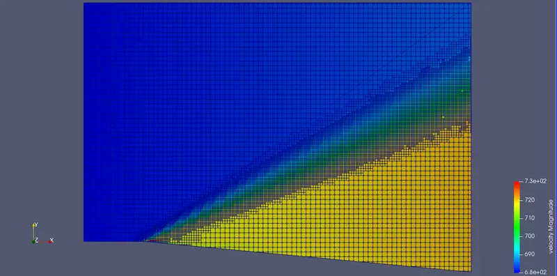
animation
Pressure plot
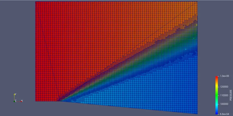
animation
Temperature plot
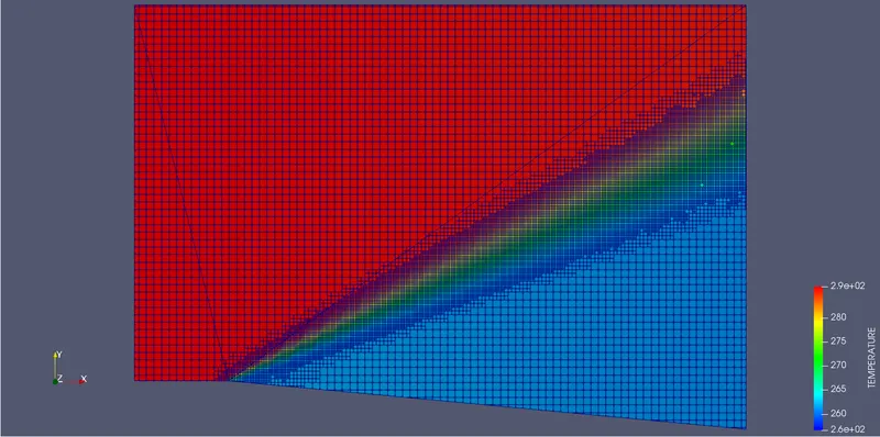
animation
Case 3:
Velocity=100m/s and SGS=0.05K
Graphical analysis:
mesh
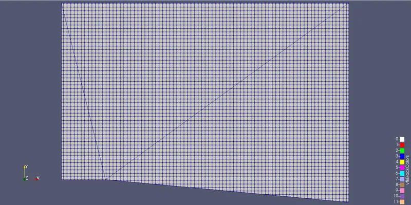
Mass flow rate:
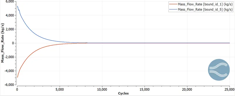
The mass flow rate conservation is followed in this case. The outlet and the inlet mass flow finally converges and conservation principle is satisfied. The initial mass flow is high 5000kg/s and starts converging at later stages of iterations. This indicates no rapid fluctuation at the bent portion of the geometry, and also other parameters remains stable, without generating any shock flow.
Average temperature:
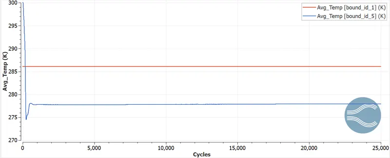
The avg temp at the outlet section is lesser than the inlet section (277.5k). At the begining of the outlet section the temperature increases to 300k but rapidly decrease because of no shock wave geneartion and no variation of other parameters.
Total average temperature:
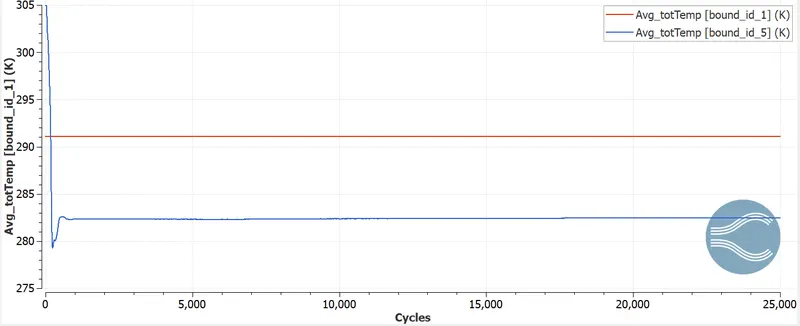
The total avg temp at the outlet section is lesser than the inlet section (277.5k). At the begining of the outlet section the temperature increases to 305k but rapidly decrease because of no shock wave geneartion and no variation of other parameters.
Static pressure:
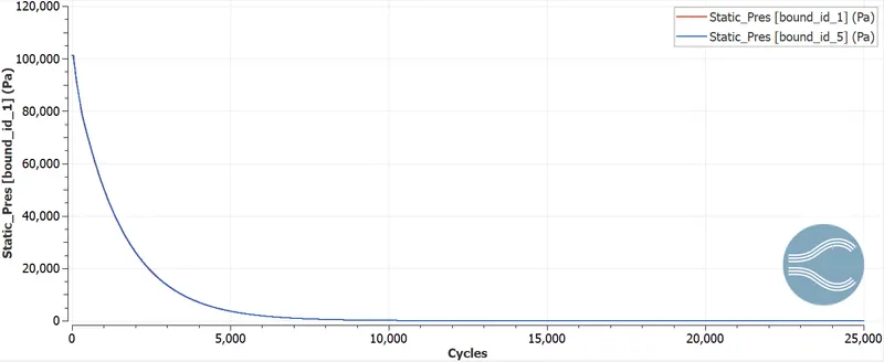
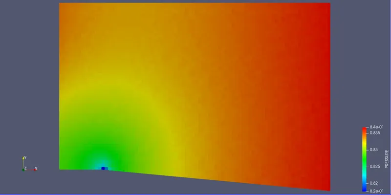
The static pressure drops to 0Pa from 1e5Pa. This is because of mass flow convergency and stability of the velocity rate, which stabilizes the pressure flow at the outlet.
Total pressure:
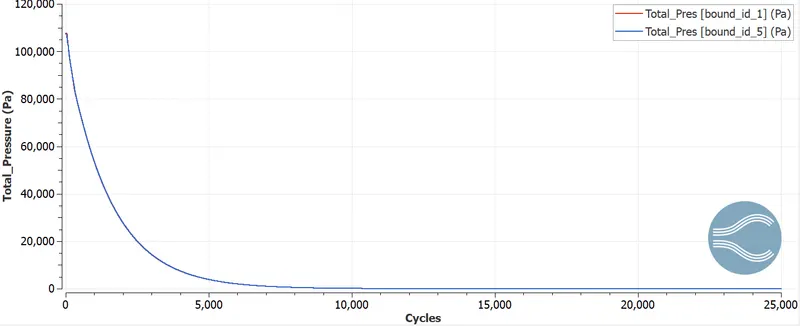
The curve of total pressure is same as that of static pressure at the inlet and outlet section. Both inlet and outlet pressure decreases due to no fluctuation genearation at the bend portion.
Mach no:
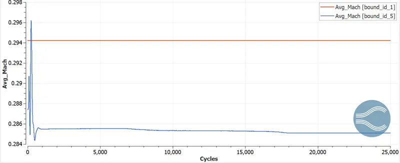
In subsonic case, the velocit is lower compared to the speed of sound. The outlet mach no is lower than that of inlet(<1), so shock waves cannot be seen. This causes the outlet velocity magnitude to be lower than the sound speed.
Cell count:
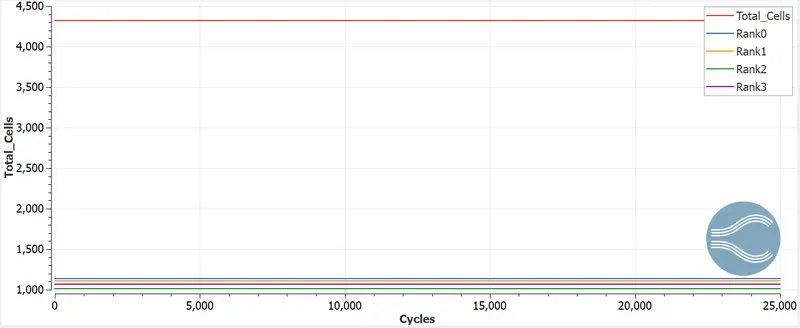
Since in this case no AMR is generated due to subsonic sped, the cel ount is als less. The overall cell count is 4300 cells. Processor0 , processor1 , processor2, processor3 have cell count in between 1000 to 1200 cells.
Velocity plot
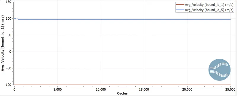
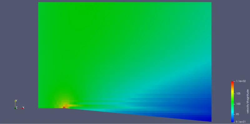
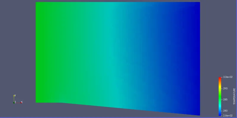
From the velocity plot, the final velocity plot has reached 100m/s and remains stable. A slight increase at the corner of the bent region is noted. Since the incoming velocity is at subsoni speed, no AMR is generated, so no shock wave to be seen.
Pressure plot
Temperature plot
Case 4:
Velocity=100m/s and SGS=0.01K
Graphical analysis:
mesh
Mass flow rate:
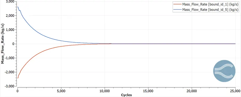
The mass flow rate conservation is followed in this case. The outlet and the inlet mass flow finally converges and conservation principle is satisfied. The initial mass flow is high 3000kg/s and starts converging at later stages of iterations. This indicates no rapid fluctuation at the bent portion of the geometry, and also other parameters remains stable, without generating any shock flow.
Average temperature:
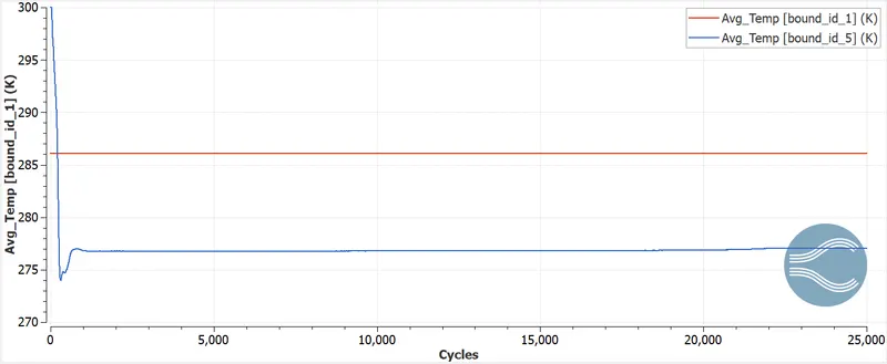
The avg temp at the outlet section is lesser than the inlet section (277.5k). At the begining of the outlet section the temperature increases to 300k but rapidly decrease because of no shock wave geneartion and no variation of other parameters.
Total average temperature:
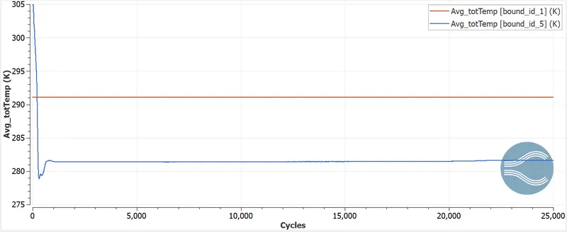
The total avg temp at the outlet section is lesser than the inlet section (277.5k). At the begining of the outlet section the temperature increases to 305k but rapidly decrease because of no shock wave geneartion and no variation of other parameters.
Static pressure:
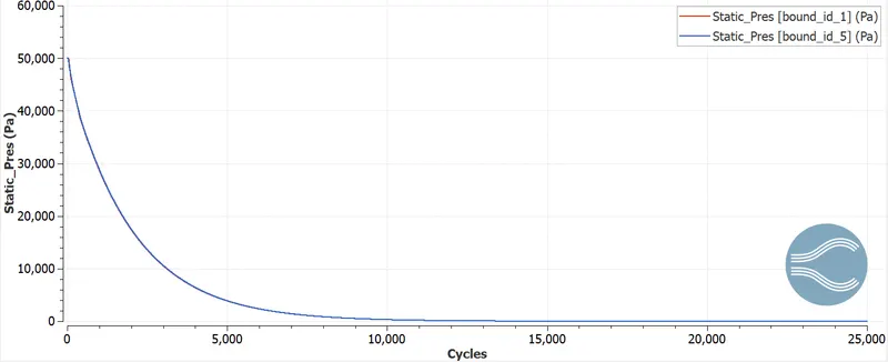
The static pressure drops to 0Pa from 1e5Pa. This is because of mass flow convergency and stability of the velocity rate, which stabilizes the pressure flow at the outlet.
Total pressure:
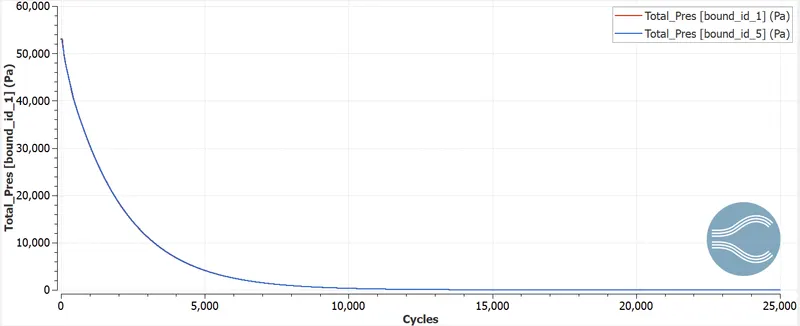
The curve of total pressure is same as that of static pressure at the inlet and outlet section. Both inlet and outlet pressure decreases due to no fluctuation genearation at the bend portion.
Mach no:
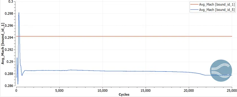
In subsonic case, the velocit is lower compared to the speed of sound. The outlet mach no is lower than that of inlet(<1), so shock waves cannot be seen. This causes the outlet velocity magnitude to be lower than the sound speed.
Cell count:
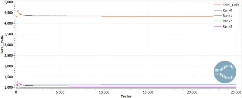
Since in this case no AMR is generated due to subsonic sped, the cel ount is als less. The overall cell count is 4300 cells. Processor0 , processor1 , processor2, processor3 have cell count in between 1000 to 1200 cells.
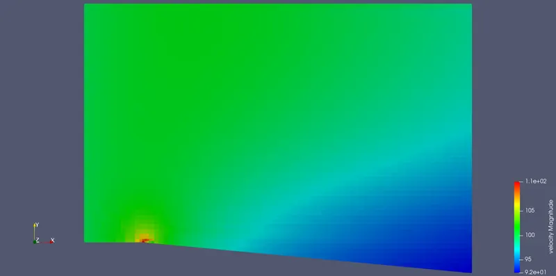
Velocity plot
From the velocity plot, the final velocity plot has reached 100m/s and remains stable. A slight increase at the corner of the bent region is noted. Since the incoming velocity is at subsoni speed, no AMR is generated, so no shock wave to be seen.
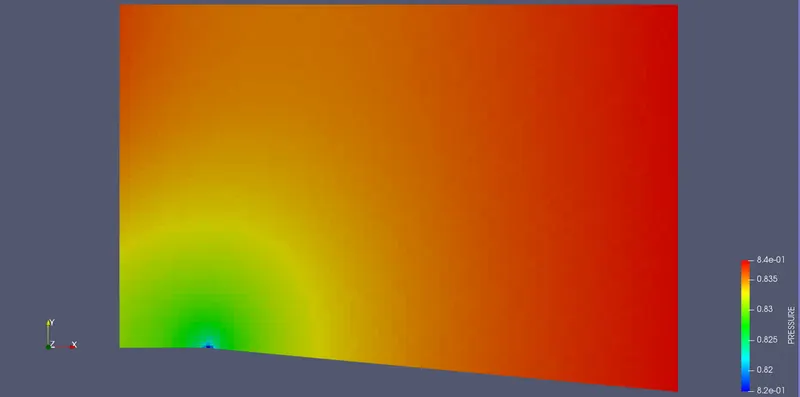
Pressure plot
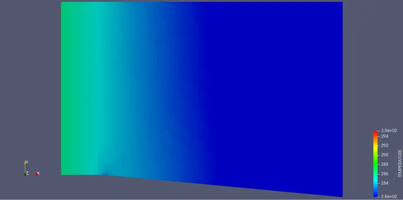
Temperature plot
Subsonic vs supersonic flow
In supersonic flow prandlt meyer expansion fan is visible and adaptive mesh refinement is done at the region of sharp turning. In case of subsonic flow, prandlt meyer expansion fan is not visible, because of no sudden fluctuation of temperature, pressure and velocity. The mach no increases in case of super sonic flow from inlet to outlet, whereas for subsonic mach no decreases.
Effect of SGS on cell count and shock location:
SGS is sub grid scaling factor, which is adaptive mesh refinement, that depends upon the gradient of parameters. On refining the cells, the details of the flow can be captured more accurately. The gradient terms refers to the second order partial derivative of temperature `(delT^2)/(delx^2)`. Suppose we define the limit of SGS for temperature to be 0.05K, then if the rise in temperature is more than the limit, the mesh gets automatically refined according to the scale. The adaptive technique helps in capturing the turbulent phenomenon.
Cell count:
As the SGS parameter decreases, the cell count increases. For small value of SGS the adaptive mesh refinement refine the cells for more no of cells in and around the shock region. Incase of supersonic speed adaptive mesh refinement starts at early stages. So the cell count increases rapidly fast. The more the refinement more is the area of cell refinement and greater the no of cell count. But in case of subsonic speed, the there is no AMR, so the no of cell count doesn't increase too much.
Shock wave location:
SGS 0.05
SGS 0.01
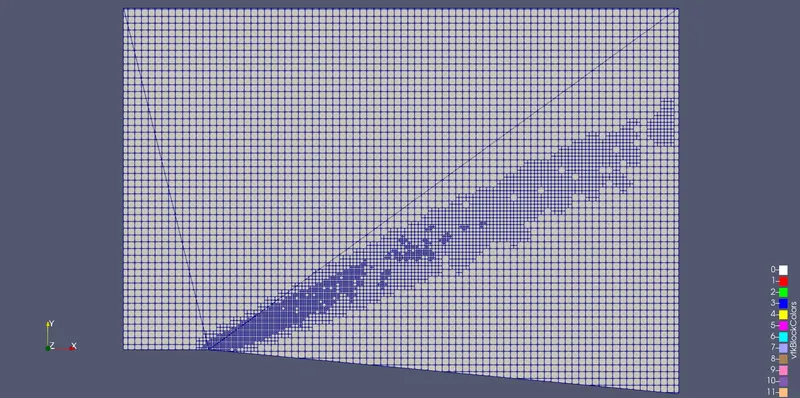
For a higher SGS value, the mesh refinement area is less. If the SGS parameter is less, the refinement is done more and the area span is greater.From the above picture we can see that for SGS value of 0.05K, the area of refinement is less and very few at the outlet section. But in case of SGS 0.01K, the prandlt meyer expansion fan is spread out across the entire region. Also the area of refinement extends upto the outlet, with large number of refinements.
In both the case the mesh refinement is done accurately to capture the shock wave and oher variation in the parameters associated with the shock wave. The accurate capture of these properties with adaptive mesh refinement technque enables us to identify the region of shock waves and its imact on the neighbouring area. For sub sonic flow no such refinement is done, and also no shock wave is produced.
Discussion:
The prandtl Meyer shock wave problem is studied using adaptive mesh refinement approach. It is found that at supersonic speed, adaptive mesh refinement is seen to change the mesh scaling at the zone of rapid fluctuation of velocity, temperature and velocity parameters. The SGS parameter decides the no of refinement to be done to effectively capture the physics of flow behaviour. With increasing the SGS scaling factor , the embedded scaling increases, also the cell cont increases and better shock wave can be seen.
In case of subsonic speed, no adaptive mesh refinement is seen, so no deviation of shock parameters ar seen. The refinement of mesh is no seen at the region of bent. The outlet parameters remains stable and no shock formation takes place. The SGS parameter also links in account of the shock location and the maximum temperature and pressure formation taken at the region.
Conclusions:
- The shock location is effectively captured by adaptive mesh refinement technique, which refines the mesh only at the region where ssubgrid scale limit exceeds.
- The pressure, temperature, mass flow and velocity changes and abruptly rises where the shock formation takes place. This ensures high high heat flow and high pressure wave generation.
- The cell count effects also depends upon the sub grid scale. higher the SGS value ore is the computational cells and more is the computational time and viceversa.
- Prandtl Meyer expansion wave is seen for supersonic flow but not for sub sonic flow. The expansion fan accounts for high mach velocity and high average temperature.