Numerical Simulation of a Super-sonic nozzle flow by MacCormack Method using MATLAB
Abstract:
Supersonic nozzles are generally used for lifting rockets and produce supersonic flows in missiles. These nozzles have converging diverging sections where the area varies from inlet section to the outlet section. In this context, a numerical simulation is performed by taking in consideration of both conservative and non-conservative forms of continuity, momentum and energy equations. The variation of mass flow rate, temperature, pressure, velocity and Mach no is observed at the steady state conditions at different time steps. Finally, a grid dependency test is performed to check the convergency criteria in both the forms of governing equations to reach the steady state solution in order to validate the analytical results.
Objectives:
- Derive both conservative and non-conservative forms of governing equations.
- Derive the steady state distribution for the flow field variables.
- Investigate the difference between two forms of governing equation and compare them.
- Plot steady state distribution of primitive variables inside the nozzle.
- Plot time wise variation of primitive variables
- Plot mass flow rate distribution inside the nozzle at various time steps during time marching process.
- Comparison of normalizes mass flow rate of both the form.
- Perform a grid independence test on the solution.
Theory and Governing equations:
The given figure represents the convergent-divergent nozzle
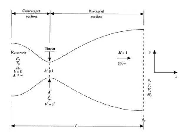
The mathematical derivation for conservative and non conservative form is described below
We start with the integral form of the continuity equation given by
`del/(del t)intintintrhodv+intintrhovdS=0`
We apply this _equation to the shaded control volume shown in Fig. This control volume is a slice of the nozzle flow, where the infinitesimal thickness of the slice is dx.
On the left side of the control volume, consistent with the quasi-one-dimensional assumption, the density, velocity, pressure, and internal energy, denoted by p, V, p, and e, respectively, are uniform over the area A. Similarly, on the right side of the control volume, the density, velocity, pressure, and internal energy, denoted by P + dp, V + dV, p + dp, and e + de, respectively, are uniform over the area A + dA. Applied to the control volume in Fig. 7.3, the volume integral becomes
`del/(delt)intintintrhodv=del/(delx)(rhoAdx)`
The surface integral in Eq. (2.19) becomes
`intintrhovdS=-rhovA+(rho+drho)(v+dv)(A+dA)`
Continuity equation
`del/(delt)(rhoA)+rhoAdel/(delx)v+rho vdel/(delx)A+Avdel/(delx)rho=0`
Momentum equation
`rhodel/(delt)v+rhovdel/(delx)v=-R(rhodel/(delx)T+Tdel/(delx)rho)`
Energy equation
`rhocvdel/(delt)T+rhovcdel/(delx)T=-rhoRT(del/(delx)v+vdel/(delx)lnA)`
Representing the above equations in non- conservation form becomes
Continuity equation
`del/(delt')rho'=-rho'del/(delx)v'-rho'v'del/(delx)lnA'-v'del/(delx)rho'`
Momentum equation
`del/(delt')v'=-v'del/(delx')v'-1/gamma(del/(delx')T'+(T')/(rho')del/(delx')rho')`
Energy equation
`del/(delt')T'=-v'del/(delx)T'-(gamma-1)T'[del/(delx)v'+v'del/(delx)lnA]`
Considering predictor steps by discretizing the equation at time step t
Continuity equation
`(del/(delt_i)rho^t)=-rho_i^t(v_(i+1)^t-v_(i)^t)/(Deltax)-rho_i^tv_i^t(lnA_(i+1)^t-lnA_(i)^t)/(Deltax)-v_i^t(rho_(i+1)^t-rho_(i)^t)/(Deltax)`
Momentum equation
`(del/(delt_i)v^t)=-v_i^t(v_(i+1)^t-v_(i)^t)/(Deltax)-1/gamma[(T_(i+1)^t-T_(i)^t)/(Deltax)+T_i^t/(rho_i^t)(rho_(i+1)^t-rho_(i)^t)/(Deltax)]`
Energy equation
`(del/(delt_i)T^t)=-v_i^t(v_(i+1)^t-v_(i)^t)/(Deltax)-(gamma-1)T_i^t[(v_(i+1)^t-v_(i)^t)/(Deltax)-v_i^t(lnA_(i+1)^t-lnA_(i)^t)/(Deltax)]`
Computing the predicted values of primitive variables of at time dt using time derivative
`ρ_i^(t+∆t)=ρ_i^t+del/(delt_i)rho^t.Deltat`
`v_i^(t+∆t)=v_i^t+del/(delt_i)v^t.Deltat`
`T_i^(t+∆t)=T_i^t+del/(delt_i)T^t.Deltat`
`∆t` is the minimum value calculated using CFL condition for all the nodes.
`Deltat=min(C*(Deltax)/(V+sonic velocity))`
Sonic velocity=`sqrt T`
Variable area cross section is given by
`A=1+2.2(x-1.5)^2,0
Moving on to the corrector step, we replace the spatial derivatives with rearward differences, using the predicted quantities. Analogously we have
Continuity equation
`(∂/(∂t)rho_i^(t+∆t))=-ρ_i^t (v_i^(t+∆t)-v_(i-1)^(t+∆t))/(∆x)-ρ_i^t v_i^t (lnA_i-lnA_(i-1))/(∆x)-v_i^t (ρ_i^(t+∆t)-ρ_(i-1)^(t+∆t))/(∆x)`
Momentum equation
`(∂/(∂t)v_i^(t+∆t))=-v_i^t (v_i^(t+∆t)-v_(i-1)^(t+∆t))/(∆x)-1/gamma [(lnT_i^(t+Deltat)-T_(i-1)^(t+Deltat))/(∆x)-(T^(t+Deltat)/(rho^(t+Deltat) )(ρ_i^(t+∆t)-ρ_(i-1)^(t+∆t))/(∆x))`
Energy equation
`(∂/(∂t)T_i^(t+∆t))=-V_i^(t+∆t) (V_i^(t+∆t)-V_(i-1)^(t+∆t))/(∆x)-(γ-1)T_i^(t+∆t) [(V_i^(t+∆t)-V_(i-1)^(t+∆t))/(∆x)+V_i^(t+∆t) (lnA_i-lnA_(i-1))/(∆x)]`
Now taking the average time derivatives of both the steps for the primitive variables
`(∂ρ/(∂t))_a=0.5(del/(delt_i)rho^t+del/(delt_i)rho^(t+dt))`
`(∂v/(∂t))_a=0.5(del/(delt_i)v^t+del/(delt_i)v^(t+dt))`
`(∂T/(∂t))_a=0.5(del/(delt_i)T^t+del/(delt_i)T^(t+dt))`
Final corrected values of primitive variables at t+ dt
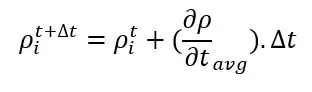
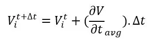
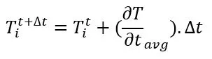
Applying the initial conditions
At timestep t= 0
`rho=1-0.3146x`
`T=1-0.2314x`
`v=(0.1+0.109x)T^(1/2)`
The use of governing equation in conservative form, we get
Conservation equation
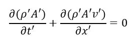
Momentum equation
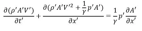
Energy equation

The equations for quasi-one-dimensional flow can be expressed in a similar generic form. Let us define the elements of the solutions vector U, the flux vector F, and the source term J as follows.
`U1=rho'A'`
`U2=rho'A'V'`
`U3=ρ^' (e^'/(γ-1)+γ/2 V^'2 )A'`
`F1=ρ^' A^' V^'`
`F2=ρ^' A^' V ' ^ 2+1/γ p'A'`
`F3=ρ^' (e^'/(γ-1)+γ/2 V^'2 ) V'A^'+p'A'V'`
With these elements, we can represent as
`del/(delt')U1=-del/(delx')F1`
`del/(delt')U2=-del/(delx')F2+J2`
`del/(delt')U3=-del/(delx')F3`
From U1, U2 and U3 we can calculate the primitive variables as
`rho'=(U1)/(A')`
`V'=(U2)/(U1)`
`'T'=e'=(gamma-1)((U3)/(U1)-gamma/2V'^2)`
`P'=rho'T'`
Pure form of the flux term
`F1=U1`
`F2=(U2^2 )/(U1)+(gamma-1)/(gamma)[U3-gamma/2((U2^2 )/(U1))]`
`F3=(gammaU2U3)/(U1)-gamma(gamma-1)/2(U2^2)/(U1^2)`
`J2=(gamma-1)/gamma(U3-gamma/2(U2^2)/(U1))del/(delx')(lnA')`
The pure form is derived to make the solution stable and converges to a steady state solution faster.
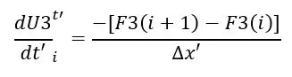
From predictor steps we get the following equation for conservative forms
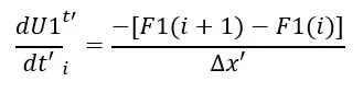
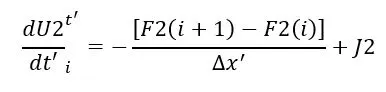
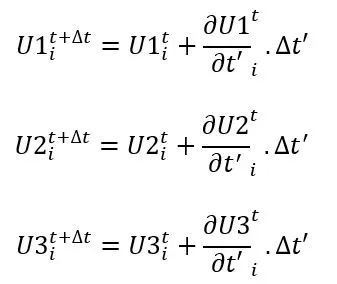
Predicted values of U1, U2 and U3 at timestep t+dt
The predicted fluxes are also obtained by replacing the updated predicted values of U1, U2, U3.
Moving on to the corrector step, we replace the spatial derivatives with rearward differences, using the predicted quantities. Analogous to predictor steps we get
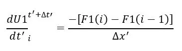
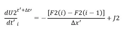
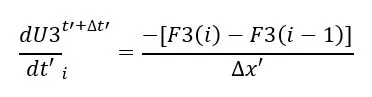
Now taking the average time derivatives of both the steps
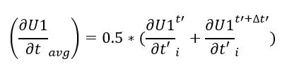
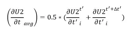
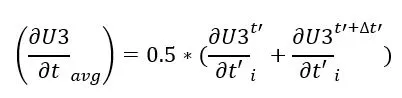
Final update of solution vectors term
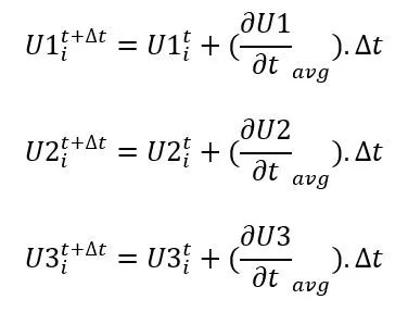
Updating the primitive variables
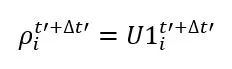
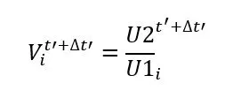
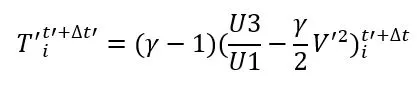
Applying the initial conditions
The present initial conditions are more realistic than those assumed in non-conservative forms
For the variation of length of nozzle, the initial conditions are defined at various domain
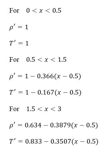
Boundary conditions
1. Non conservative form
Applying boundary conditions
Inlet
At subsonic condition inlet density and temperature is fixed, and velocity is allowed to float
v(1)= 2*v(2) – v(3)
Outlet
At supersonic condition all the flow variables are allowed to float
`rho(n)=2rho(n-1)-rho(n-2)`
`T(n)=2T(n-1)-T(n-2)`
`V(n)=2V(n-1)-V(n-2)`
2.Conservative form
The boundary conditions for the subsonic-supersonic isentropic flow solution using the conservation form of the governing equations are theoretically the same as non -conservative form
At inlet density and temperature is fixed and velocity is allowed to float
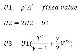
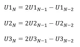
At oulet of supersonic outflow
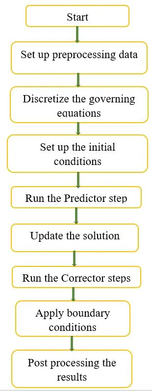
Workflow of the problem
Algorithm
- In the main program code, define the no of grid points, length of nozzle, mesh size and grid point at throat.
- A function calls for both conservative and non-conservative form are defined.
- Inside the conservative function, the initial conditions set up are defined within the flow domain.
- Define the primitive variables, sonic velocity, courant no and solution vectors.
- Starting with time marching step, the flux terms are defined inside the time loop.
- Inside time loop a nodal loop is defined for inner nodes of nozzle. The predictor step is followed by updating the solution vector terms and the primitive variables.
- In the next spatial loop corrector step is executed with the new predicted values of solution vectors and flux terms.
- With finally taking the average values of predictor and corrector steps, the boundary conditions are applied.
- With each time step the mass flow rate is observed over the entire length of nozzle. The transient effect at the throat section is also captured.
- A similar approach for non-conservation is followed from step3 to step 9.
- In the main program, variation of primitive variables at the throat section is plotted to observe the steady state approach. Also, temperature, pressure and density variation across the entire domain of nozzle for different forms of equation are plotted.
MATLAB code
Main program code
clc
clear all
close all
%inputs
n=31;  %no of grid points
x=linspace(0,3,n);% length of the domain
dx=x(2)-x(1);% grid spacing in x domain
courant_no=0.5;% define the CFL criteria
throat=(n-1)/2+1;% define the grid point at the throat
area=1+(2.2*(x-1.5).^2);%define the area of the nozzle
gamma=1.4;%ratio of cp/cv
nt=1400;% no of time step
% %----------------------------------------------------------------------------------------------
%%%%%%%%%%%%%%%%%%% function call for conservative and non conservative forms%%%%%%
tic
[rho_c, p_c, T_c, v_c, mass_flow_c,mach_no_c,p_t_c,Temp_t_c, v_t_c, mach_t_c, rho_t_c,dU1_dt_t,dU2_dt_t,dU3_dt_t]=conservative_form(n,x,dx,courant_no,throat,gamma,area,nt);
time_c=toc;

tic
[rho_nc, p_nc, T_nc, v_nc, mass_flow_nc,mach_no_nc,p_t_nc,Temp_t_nc, v_t_nc, mach_t_nc, rho_t_nc, drhodt_t,dvdt_t,dTdt_t]=nonconservative_form(n,x,dx,courant_no,throat,gamma,area,nt);
time_nc=toc;

%-------------------------------------------------------------------------%
%-------------------plot for primitive variables in conservative part--------------------------
figure(1)
suptitle('conservative form')
subplot(3,1,1)
plot(x,rho_c,'-*','color','b','linewidth',1.5)
legend('density')
xlabel('length of domain')
ylabel('{rho/rho0}')
grid on
subplot(3,1,2)
plot(x,p_c,'-*','color','r','linewidth',1.5)
legend('pressure')
xlabel('length of domain')
ylabel('P/P0')
grid on
subplot(3,1,3)
plot(x,T_c,'-*','color','m','linewidth',1.5)
legend('Temperature')
xlabel('length of domain')
ylabel('T/T0')
grid on
y=table(x', rho_c', p_c', T_c', v_c', mach_no_c', mass_flow_c');% table representing the steady state solution for conservative approach

%-------------------plot for primitive variables in the transient throat section of nozzle--------
figure(2)
suptitle('conservation form variables at transient throat section')
subplot(5,1,1)
plot(rho_t_c,'color','b','linewidth',1.5)
legend('density at throat section')
xlabel('no of timesteps taken to converge')
ylabel('{rho}(density)')
grid on
subplot(5,1,2)
plot(p_t_c,'color','y','linewidth',1.5)
legend('Pressure at throat section')
xlabel('no of timesteps taken to converge')
ylabel('Pressure')
grid on
subplot(5,1,3)
plot(Temp_t_c,'color','r','linewidth',1.5)
legend('Temperature at throat section')
xlabel('no of timesteps taken to converge')
ylabel('Temperature')
grid on
subplot(5,1,4)
plot(v_t_c,'color','g','linewidth',1.5)
legend('Velocity at throat section')
xlabel('no of timesteps taken to converge')
ylabel('Velocity')
grid on
subplot(5,1,5)
plot(mach_t_c,'color','m','linewidth',1.5)
legend('Mach no at throat section')
xlabel('no of timesteps taken to converge')
ylabel('Mach no')
grid on
% %----------------------residuals for  conservative form----------------
figure(3)
title('Residuals for conservative forms')
plot( dU1_dt_t,'color','b','linewidth',1.5)
xlabel('no of timesteps taken to converge')
hold on
plot( dU2_dt_t,'color','r','linewidth',1.5)
hold on
plot( dU3_dt_t,'color','m','linewidth',1.5)
legend('residual in throat section for U1','residual in throat section for U2','residual in throat section for U3')
xlabel('no of timesteps taken to converge')
ylabel('Residual')
title('Residuals for conservative forms')
%-----------------------------------------------------------------------
%-------------------plot for primitive variables in non-conservative part--------------------------
figure(4)
suptitle('Non conservative form')
subplot(3,1,1)
plot(x,rho_nc,'-*','color','b','linewidth',1.5)
legend('density')
xlabel('length of domain')
ylabel('{rho/rho0}')
grid on
subplot(3,1,2)
plot(x,p_nc,'-*','color','r','linewidth',1.5)
legend('Pressure')
xlabel('length of domain')
ylabel('P/P0')
grid on
subplot(3,1,3)
plot(x,T_nc,'-*','color','m','linewidth',1.5)
legend('Temperature')
xlabel('length of domain')
ylabel('T/T0')
grid on
z=table(x', rho_nc', p_nc', T_nc', v_nc', mach_no_nc', mass_flow_nc');% table representing the steady state solution for non conservative approach

%-------------------plot for primitive variables in the transient throat section of nozzle--------
figure(5)
suptitle('Non conservation form variables at transient throat section')
subplot(5,1,1)
plot(rho_t_nc,'color','b','linewidth',1.5)
legend('density at throat section')
xlabel('no of timesteps taken to converge')
ylabel('{rho}(density')
grid on
subplot(5,1,2)
plot(p_t_nc,'color','y','linewidth',1.5)
legend('Pressure at throat section')
xlabel('no of timesteps taken to converge')
ylabel('Pressure')
grid on
subplot(5,1,3)
plot(Temp_t_nc,'color','r','linewidth',1.5)
legend('Temperature at throat section')
xlabel('no of timesteps taken to converge')
ylabel('Temperature')
grid on
subplot(5,1,4)
plot(v_t_nc,'color','g','linewidth',1.5)
legend('Velocity at throat section')
xlabel('no of timesteps taken to converge')
ylabel('Velocity')
grid on
subplot(5,1,5)
plot(mach_t_nc,'color','m','linewidth',1.5)
legend('Mach no at throat section')
xlabel('no of timesteps taken to converge')
ylabel('Mach no')
grid on
% %----------------------residuals for non conservative form----------------
figure(6)
plot( drhodt_t,'color','b','linewidth',1.5)
legend('residual in throat section for density')
hold on
plot( dvdt_t,'color','r','linewidth',1.5)
legend('residual in throat section for velocity')
hold on
plot( dTdt_t,'color','m','linewidth',1.5)
legend('residual in throat section for density','residual in throat section for velocity','residual in throat section for temperature')
xlabel('no of timesteps taken to converge')
ylabel('Residual')
title('Residuals for non conservative forms')
% %----------------------comparison between conservative and non conservative form----------------
figure (7)
plot(x,mass_flow_c,'linewidth',1.5)
hold on
plot(x,mass_flow_nc,'linewidth',1.5)
legend('conservative mass flow rate','non conservative mass flow rate')
xlabel('length of domain')
ylabel('mass flow rate')
% %-------------------------------------------------------------------------------
figure (8)
plot(x,rho_nc,'-*','linewidth',1.5)
hold on
plot(x,mach_no_nc,'-*','linewidth',1.5)
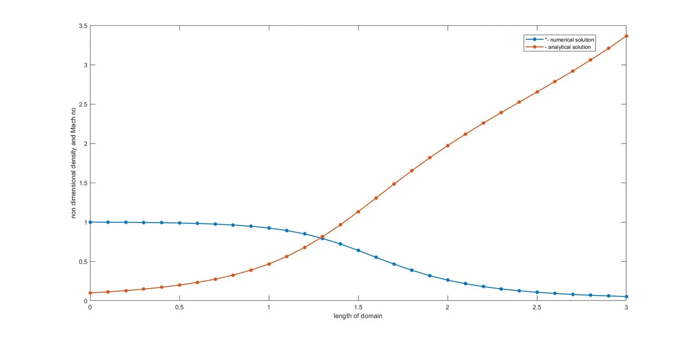
legend('*- numerical solution','- analytical solution')
xlabel('length of domain')
ylabel('non dimensional density and Mach no')
function call for conservative form
function [rho, p, T, v, mass_flow,mach_no,p_t,Temp_t, v_t, mach_t, rho_t,dU1_dt_t,dU2_dt_t,dU3_dt_t]=conservative_form(n,x,dx,courant_no,throat,gamma,area,nt)

%--------------------------initial conditions---------------------------
for i=1:length(x)
    if (x(i)>=0&&x(i)<=0.5)
        rho(i)=1;
        T(i)=1;
    else
        if (x(i)>0.5&&x(i)<=1.5)
            rho(i)=1-0.366*(x(i)-0.5);
            T(i)=1-0.167*(x(i)-0.5);
        else
            if(x(i)>1.5&&x(i)<=3)
                rho(i)=0.634-0.3879*(x(i)-1.5);
                T(i)=0.833-0.3507*(x(i)-1.5);
            end
        end
    end
end
%-------------------------------------------------------------------------%

%-----------------------define the primitive variables--------------------%
v=0.59./(rho.*area);% velocity terms
p=rho.*T;% pressure terms
a=sqrt(T);% sonic velocity
dt=min(courant_no*dx./(a+v));% minimum time step

%-----------------------define the solution vectors--------------------%
U1=rho.*area; % continuity equation
U2=rho.*area.*v;% momentum equation
U3=rho.*((T/(gamma-1))+(gamma/2)*v.^2).*area;% energy equation


for i=1:nt% time marching loop

 U1_old=U1;
 U2_old=U2;
 U3_old=U3;
  %----------------------define the flux terms----------------------------
F1=U2;
f2=((gamma-1)/gamma)*(U3-((gamma/2)*(U2.^2./U1)));
F2=(U2.^2./U1)+f2;
F3=(gamma*(U2.*U3)./U1)-((gamma*(gamma-1)/2)*(U2.^3./U1.^2));


 for j=2:n-1%space marching for the inner nodes in predictor step
   %--------------------------defining the source term in predictor step--------
J2(j)= (1/gamma)*rho(j)*T(j)*(area(j+1)-area(j))/dx;
  %--------------------------predictor step marching-------------------------------
 dU1_dt_p(j)=-(F1(j+1)-F1(j))/dx;
 dU2_dt_p(j)=-((F2(j+1)-F2(j))/dx)+J2(j);
 dU3_dt_p(j)=-(F3(j+1)-F3(j))/dx;

%--------------------------update the solution vector terms-------------------
  U1(j)=U1(j)+(dU1_dt_p(j)*dt);
  U2(j)=U2(j)+(dU2_dt_p(j)*dt);
  U3(j)=U3(j)+(dU3_dt_p(j)*dt);
 end


%  %--------------------------update the primitive terms-------------------
  rho=U1./area;
  v=U2./U1;
  T=(gamma-1)*((U3./U1)-((gamma/2)*v.^2));
 %--------------------------update the flux terms-------------------
  F1=U2;
  f2=((gamma-1)/gamma)*(U3-((gamma/2)*(U2.^2./U1)));
  F2=(U2.^2./U1)+f2;
  F3=(gamma*(U2.*U3)./U1)-(gamma*(gamma-1)/2)*(U2.^3./U1.^2);


 for j=2:n-1%space marching for the inner nodes i corrector steps
 %-----------------defining the source term in corrector steps-------------
    m(j)= (1/gamma)*rho(j)*T(j)*(area(j)-area(j-1))/dx;
%  %--------------------------corrector step marching---------------------
   dU1_dt_c(j)=-(F1(j)-F1(j-1))/dx;
   dU2_dt_c(j)=-((F2(j)-F2(j-1))/dx)+m(j);
   dU3_dt_c(j)=-(F3(j)-F3(j-1))/dx;

  end
%  %-------------------average of predictor and corrector steps------------
   dU1_dt=0.5*(dU1_dt_p+dU1_dt_c);
   dU2_dt=0.5*(dU2_dt_p+dU2_dt_c);
   dU3_dt=0.5*(dU3_dt_p+dU3_dt_c);


%  %--------------------------update the solution vectors terms--------------
  for j=2:n-1%space marching for updating solution vectors at inner nodes
 U1(j)=U1_old(j)+(dU1_dt(j)*dt);
 U2(j)=U2_old(j)+(dU2_dt(j)*dt);
 U3(j)=U3_old(j)+(dU3_dt(j)*dt);

 end
%------------------------------ applying boundary conditions-----------------------
% inlet boundary conditions
rho(1)=1;
T(1)=1;
U1(1)=rho(1)*area(1);
U2(1)=2*U2(2)-U2(3);
v(1)=U2(1)/U1(1);
U3(1)=U1(1)*((T(1)/(gamma-1))+(gamma/2)*(v(1)^2));

% outlet boundary conditions
U1(n)=2*U1(n-1)-U1(n-2);
U2(n)=2*U2(n-1)-U2(n-2);
U3(n)=2*U3(n-1)-U3(n-2);
%  %--------------------------update the primitive term-------------------

 rho=U1./area;
 v=U2./U1;
 T=(gamma-1)*((U3./U1)-((gamma/2)*v.^2));
 p=rho.*T;
 mach_no=v./a;
 mass_flow=U2;

%---------------------computing the primitive variables at the transient throat section-----------------
  rho_t(i)=rho(throat);
  mach_t(i)=mach_no(throat);
  Temp_t(i)=T(throat);
  v_t(i)=v(throat);
  p_t(i)=p(throat);
% %----------------residue at throat section-------------------------------
  dU1_dt_t(i)=dU1_dt(throat);
  dU2_dt_t(i)=dU2_dt(throat);
  dU3_dt_t(i)=dU3_dt(throat);
% %--------------------------------------------------------------

% ----------------------plot for mass flow rate at different time steps----------
  figure (14)

  if i==10
      plot(x,mass_flow,'-x','linewidth',1.5)
         hold on
     else
          if i==50
          plot(x,mass_flow,'-*','linewidth',1.5)
         hold on
         else
              if i==200
            plot(x,mass_flow,'-p','linewidth',1.5)
         hold on
              else
               if i==400
            plot(x,mass_flow,'-h','linewidth',1.5)
   legend('10{Delta}t','50{Delta}t','200{Delta}t','400{Delta}t')
 xlabel('length of domain')
 ylabel('mass flow rate variation at different time steps')
 title('Mass flow at different time steps for conservative forms')
 axis([0 3 0 2])

    else
 end
 end
 end
 end

end
end
function call for Non conservative form
function [rho, p, T, v, mass_flow,mach_no,p_t,T_t, v_t, mach_t, rho_t, drhodt_t,dvdt_t,dTdt_t ]=nonconservative_form(n,x,dx,courant_no,throat,gamma,area,nt);


%--------------------------initial conditions------------------------
rho=1-0.3146.*x;
T=1-(0.2314.*x);
v=(0.1+1.09.*x).*T.^0.5;

%---------------------------define the primitive variables--------------
a=sqrt(T);
dt=min(courant_no*dx./(a+v));
p=rho.*T;
mach_no=a./v;
%--------------------------------------------------------------------

for i=1:nt%time marching loop

    rho_old=rho;
    v_old=v;
    T_old=T;

%------------------------------predictor step marching------------------

 for j=2:n-1%space marching for the inner nodes in predictor step

     dvdx=[v(j+1)-v(j)]/dx;
     drhodx=[rho(j+1)-rho(j)]/dx;
     dTdx=[T(j+1)-T(j)]/dx;
     dlog_a_dx=[log(area(j+1))-log(area(j))]/dx;

%-------------continuity equation----------

 drhodt_p(j)=-rho(j)*dvdx-rho(j).*v(j).*dlog_a_dx-v(j).*drhodx;
 %------------momentum equation-----------
 dvdt_p(j)=-v(j).*dvdx-(1/gamma).*(dTdx+(T(j)./rho(j)).*drhodx);
 %------------energy equation---------------
 dTdt_p(j)=-v(j).*dTdx-(gamma-1).*T(j).*(dvdx+v(j).*dlog_a_dx);

 %----------------update primitive variables in predictor steps------------

 rho(j)=rho(j)+drhodt_p(j)*dt;
 v(j)=v(j)+dvdt_p(j)*dt;
 T(j)=T(j)+dTdt_p(j)*dt;

  p=rho.*T;
  mach_no=v./a;
 mass_flow=rho.*area.*v;
 %-----------------------------------------------------------------------
 end

 %----------------------------corrector step marching------------------

 for j=2:n-1%space marching for the inner nodes in corrector step

     dvdx=[v(j)-v(j-1)]/dx;
     drhodx=[rho(j)-rho(j-1)]/dx;
     dTdx=[T(j)-T(j-1)]/dx;
     dlog_a_dx=[log(area(j))-log(area(j-1))]/dx;

%-------------continuity equation----------

 drhodt_c(j)=-rho(j).*dvdx-rho(j).*v(j)*dlog_a_dx-v(j).*drhodx;
 %------------momentum equation-----------
 dvdt_c(j)=-v(j)*dvdx-(1/gamma)*(dTdx+(T(j)/rho(j))*drhodx);
 %------------energy equation---------------
 dTdt_c(j)=-v(j)*dTdx-(gamma-1)*T(j)*(dvdx+v(j)*dlog_a_dx);
 %---------------------------------------------------------------------

 end

 %--------------------average of predictor and corrector steps--------

 drhodt=0.5*(drhodt_p+drhodt_c);
 dvdt=0.5*(dvdt_p+dvdt_c);
 dTdt=0.5*(dTdt_p+dTdt_c);
 %------------------------------------------------------------------

 %-----------------------final solution update for primitive variables--------------
 for j=2:n-1
  rho(j)=rho_old(j)+drhodt(j)*dt;
  v(j)=v_old(j)+dvdt(j)*dt;
  T(j)=T_old(j)+dTdt(j)*dt;
 end
 mass_flow=rho.*area.*v;

 %-----------------------applying boundary conditions----------------------

 %---------inlet boundary conditions-----------
 v(1)=2*v(2)-v(3);

 %---------outlet boundary conditions----------

 v(n)=2*v(n-1)-v(n-2);
 rho(n)=2*rho(n-1)-rho(n-2);
 T(n)=2*T(n-1)-T(n-2);

%---------------------computing the primitive variables at the transient throat section--------------
rho_t(i)=rho(throat);
v_t(i)=v(throat);
T_t(i)=T(throat);
mass_t(i)=rho(throat)*v(throat)*area(throat);
p_t(i)=p(throat);
mach_t(i)=mach_no(throat);
% %----------------residue at throat section-------------------------------
drhodt_t(i)= drhodt(throat);
dvdt_t(i)=dvdt(throat);
dTdt_t(i)=dTdt(throat);
% ----------------------plot for mass flow rate at different time steps----------
if i==1
    figure (13)
    plot(x,mass_flow,'-o','linewidth',1.5)
    hold on
else
    if i==50

   plot(x,mass_flow,'->','linewidth',1.5)
  hold on
    else
        if i==100

       plot(x,mass_flow,'-^','linewidth',1.5)
        else
        if i==150

       plot(x,mass_flow,'-*','linewidth',1.5)
       else
            if i==500
       plot(x,mass_flow,'-s','linewidth',1.5)
            else
        if i==700
       plot(x,mass_flow,'-+','linewidth',1.5)
        else
            if i==1000

       plot(x,mass_flow,'-p','linewidth',1.5)
            else
            if i==1400
       plot(x,mass_flow,'-h','linewidth',1.5)
            else
     legend('1{Delta}t','50{Delta}t','100{Delta}t','150{Delta}t','500{Delta}t','700{Delta}t','1000{Delta}t','1400{Delta}t')
     xlabel('length of domain')
     ylabel('mass flow rate at different time steps')
     title('Mass flow at different time steps for non conservative forms')
end
end
end
end
end
end
end
end


end
end
Results and analysis
1. Conservative form of equation
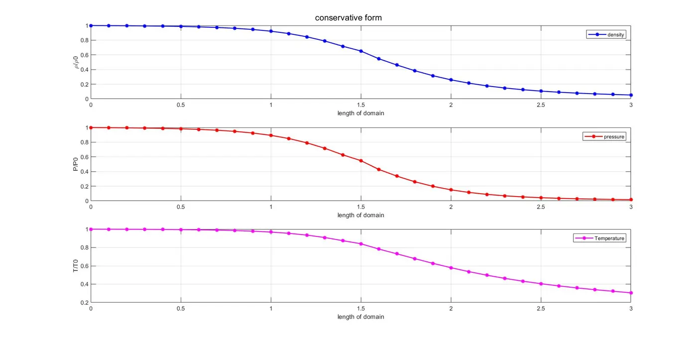
As seen for conservative form, the magnitude of primitive variables reduces from inlet to the outlet of nozzle. This predicts the convergence towards the steady state condition.
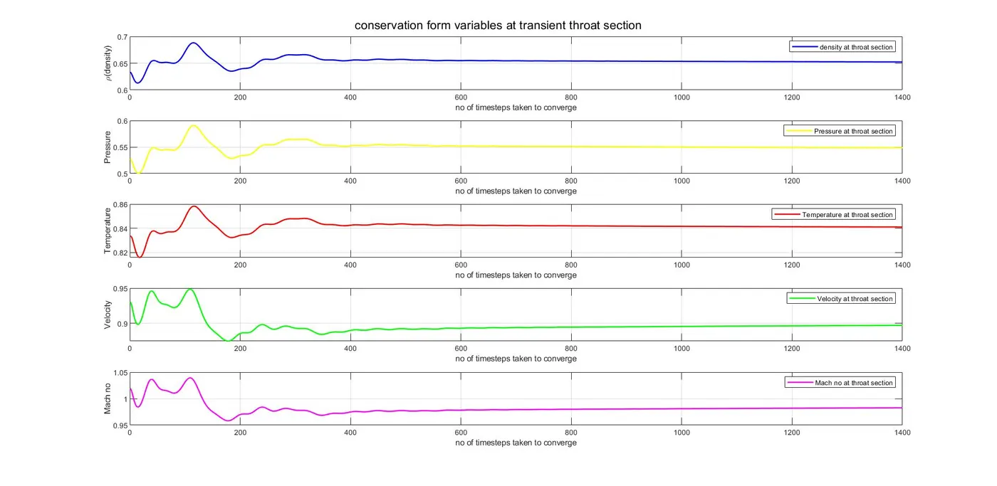
Time wise variation of flow field variables
The largest change take place at the early times after which the final steady state value reaches asymptotically. At steady state the approach becomes more relaxed and gradually approaches to steady state solution. The steady state approach is reached 600 timestep of iterations.
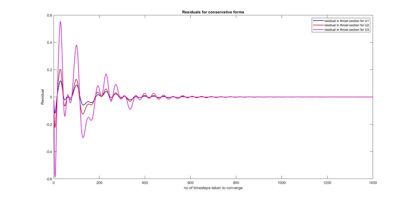
Residual plot for conservation
At early times, the time derivatives are large and they oscillate in value. These oscillations are associated with various unsteady compression and expansion waves which propagated through the nozzle during transient process.
At later stages, the derivatives rapidly grow small, changing over the span of 1000 steps. The steady state for conservation is reached after 600-time steps and for non-conservation after 500-time step.
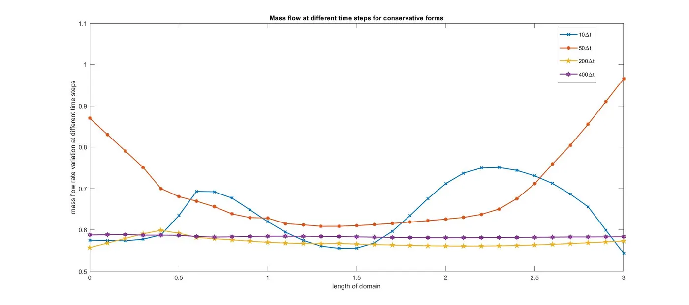
Mass flow variation in conservation form
At the beginning of time step at 10-∆t the variation becomes sinusoidal in nature. After 50-∆t the mass flow changes to parabolic like curvature. After 200-∆t the mass flow variation converges and attains steady state conditions.
The fluctuation in mass flow rate is also minimum than that observed in non- conservational approach.
2.Non conservative form of equation
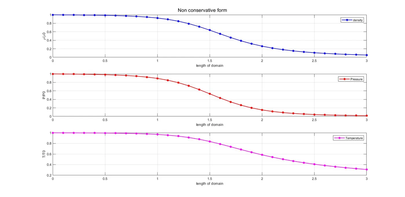
The pattern is similar to conservative form, Only the difference is that in non-conservation the steady state condition reaches faster than conservation due to rapid change in residual.
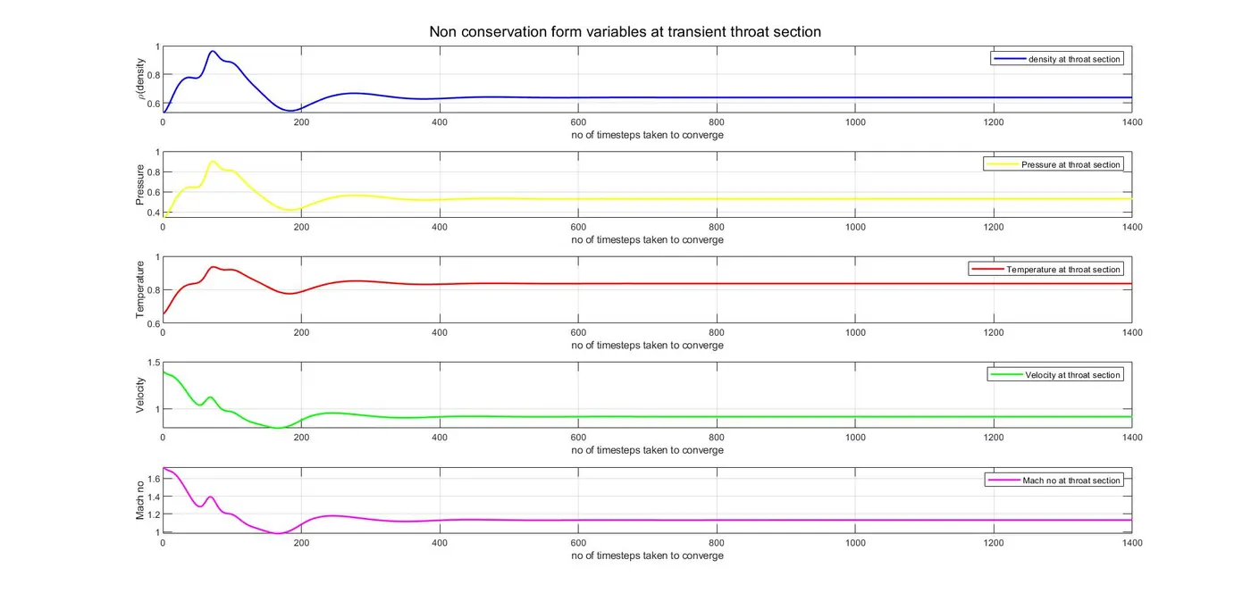
Time wise variation of flow field variables
In case of non-conservation form the fluctuation of primitive variables at the beginning of time step is less compared to conservative form. after 400 time step it easily attains steady state profile.
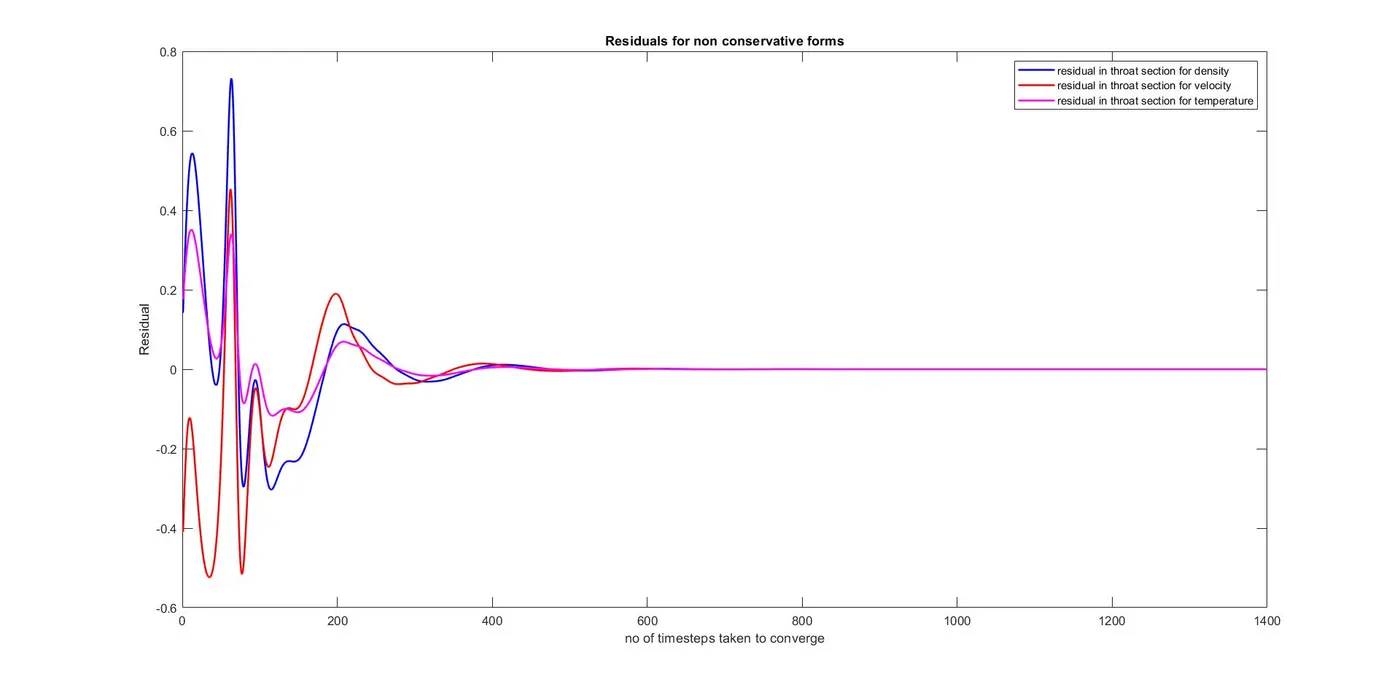
Residual plot for non-conservation
The fluctation dies ot as the derivative grow smaller at afaster rate than conservative form. On reaching 200 time step the oscillation settles down and converges to steady state condition.
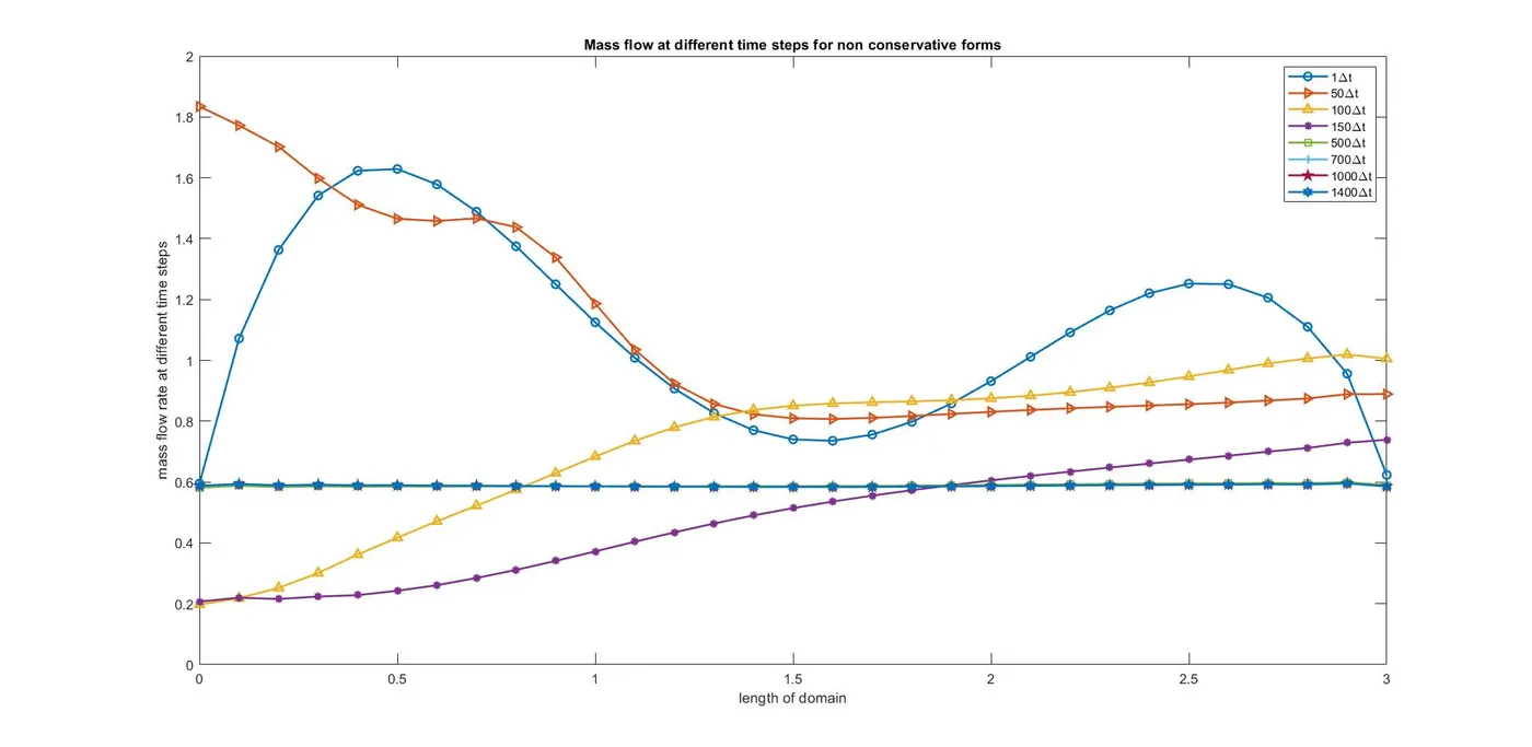
Mass flow variation in non-conservation form
The __o__ line pertains to initial condition 1∆t. after 50time steps, the mass flow variation changes to sine wave distributions. At 100 ∆t - it starts flopping and. After 200-∆t it starts to settle down. At 700∆t it starts converging and at 1000∆t mass flow gets completely converges to steady state.
3.Comparison between conservative and non conservative form
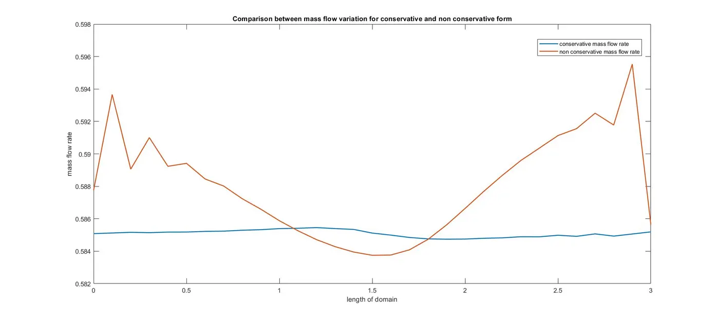
The conservation form preserves the mass flow rate much better than non-conservation form. This is because mass flow itself is one of dependent variables in conservation form. In non-conservation, the mass flow is obtained as a secondary result.
In non-conservation form the mass flow rate is higher at the initial and final phase and lowest at the mid-section of the nozzle. This shows instability in mass flow rate. But in case of conservation, a small variation is observed at throat section and at other section of nozzle it is same.
Outputs
1.Steady state solution for conservative form
|
x/L |
density |
pressure |
temperature |
velocity |
Mach no |
Mass flow rate |
|
0 |
1 |
1 |
1 |
0.0983334779678854 |
0.0983334779678854 |
0.585084193908918 |
|
0.100000000000000 |
0.998747453983239 |
0.998260784923430 |
0.999512720600320 |
0.110289585703655 |
0.110289585703655 |
0.585124464803744 |
|
0.200000000000000 |
0.997093229343798 |
0.995936383203946 |
0.998839781370682 |
0.124389706239206 |
0.124389706239206 |
0.585164735698569 |
|
0.300000000000000 |
0.994864885775526 |
0.992837688494873 |
0.997962339097863 |
0.141114160857332 |
0.141114160857332 |
0.585143534042360 |
|
0.400000000000000 |
0.991847953697617 |
0.988616333555777 |
0.996741819015916 |
0.161111129602045 |
0.161111129602045 |
0.585179339310570 |
|
0.500000000000000 |
0.987687875584530 |
0.982835056645054 |
0.995086687748795 |
0.185149195010682 |
0.185149195010682 |
0.585182768276118 |
|
0.600000000000000 |
0.981920833000549 |
0.974803637771560 |
0.992751762678016 |
0.214233814309012 |
0.216045388468156 |
0.585223315511673 |
|
0.700000000000000 |
0.973804872684924 |
0.963565154949249 |
0.989484836210110 |
0.249576561726769 |
0.253851890463525 |
0.585237603577286 |
|
0.800000000000000 |
0.962329697131944 |
0.947698568109845 |
0.984796136848209 |
0.292687780668749 |
0.300307132940520 |
0.585293933829721 |
|
0.900000000000000 |
0.946005800907369 |
0.925285491166766 |
0.978097058473924 |
0.345276586895130 |
0.357420752561017 |
0.585327508183560 |
|
1 |
0.922902888458893 |
0.893766398377508 |
0.968429516858444 |
0.409222943765690 |
0.427458286494874 |
0.585393207078760 |
|
1.10000000000000 |
0.890559432440843 |
0.850173286342285 |
0.954650813154752 |
0.486210916734315 |
0.512568261899757 |
0.585415618808269 |
|
1.20000000000000 |
0.846464438538682 |
0.791647470776353 |
0.935240081843292 |
0.577336251140073 |
0.614361349188590 |
0.585456137591832 |
|
1.30000000000000 |
0.788743016046847 |
0.716843827374793 |
0.908843327662779 |
0.682158083408119 |
0.732868082572289 |
0.585395597451325 |
|
1.40000000000000 |
0.717580295259428 |
0.627505551827377 |
0.874474335447734 |
0.798159540567794 |
0.865878388291937 |
0.585343917078032 |
|
1.50000000000000 |
0.652367411539514 |
0.548660224337477 |
0.841029479143817 |
0.896915779035696 |
0.982718572093062 |
0.585118625138464 |
|
1.60000000000000 |
0.547002820586239 |
0.428274799082332 |
0.782948063454841 |
1.04643077434031 |
1.17146173286358 |
0.584993397984862 |
|
1.70000000000000 |
0.461746549124898 |
0.337518954293369 |
0.730961508933927 |
1.16415407031489 |
1.33287075532406 |
0.584848007583953 |
|
1.80000000000000 |
0.383604590979635 |
0.260180524336679 |
0.678251852179974 |
1.27244143907209 |
1.49153951036400 |
0.584761024581384 |
|
1.90000000000000 |
0.315948741928583 |
0.198205353915523 |
0.627333891901763 |
1.36889542988366 |
1.64471786686466 |
0.584741066597570 |
|
2 |
0.259622523009349 |
0.150536688004030 |
0.579829077458772 |
1.45310366367460 |
1.79183982763320 |
0.584750581003859 |
|
2.10000000000000 |
0.213886763989511 |
0.114758551389643 |
0.536538817312093 |
1.52575132354158 |
1.93368697900948 |
0.584797719735082 |
|
2.20000000000000 |
0.177205556889727 |
0.0881870624086498 |
0.497654046275353 |
1.58819038534451 |
2.07202471324973 |
0.584824343974953 |
|
2.30000000000000 |
0.147949189168290 |
0.0685031951649140 |
0.463018388610379 |
1.64175020745646 |
2.20884133853016 |
0.584892633720214 |
|
2.40000000000000 |
0.124550986736436 |
0.0538359365919826 |
0.432240145201785 |
1.68798762177628 |
2.34675977988043 |
0.584889137465111 |
|
2.50000000000000 |
0.105803297783849 |
0.0428473140433327 |
0.404971441730178 |
1.72780631561353 |
2.48792008499342 |
0.584984339595754 |
|
2.60000000000000 |
0.0906108269461052 |
0.0344881670072255 |
0.380618610044679 |
1.76277157850941 |
2.63590998727090 |
0.584917309412626 |
|
2.70000000000000 |
0.0782969551226707 |
0.0281196439512521 |
0.359140964130675 |
1.79280919840251 |
2.79255124292866 |
0.585068417630270 |
|
2.80000000000000 |
0.0681109781252526 |
0.0231186543605693 |
0.339426256925209 |
1.82024708997746 |
2.96420228443286 |
0.584932024296750 |
|
2.90000000000000 |
0.0597671937062846 |
0.0192926647761117 |
0.322796898762256 |
1.84281211283241 |
3.15105008992337 |
0.585062131615438 |
|
3 |
0.0527090875866598 |
0.0161006220066261 |
0.305461975226850 |
1.86593320618480 |
3.36792393718483 |
0.585192238934126 |
2.Steady state solution for non conservative form
|
x/L |
density |
pressure |
temperature |
velocity |
Mach no |
Mass flow rate |
|
0 |
1 |
1 |
1 |
0.0987829235631804 |
0.0987829235411876 |
0.587758395070066 |
|
0.100000000000000 |
0.997798718088226 |
0.996956410788363 |
0.999114629654295 |
0.112004394038148 |
0.113177663738610 |
0.593657650284513 |
|
0.200000000000000 |
0.997030649471058 |
0.995418964865800 |
0.998810799333307 |
0.125225864513115 |
0.128349585212683 |
0.589061290073071 |
|
0.300000000000000 |
0.994272068768540 |
0.991759592378697 |
0.997702073373663 |
0.142611974350165 |
0.147800099022542 |
0.591001988338294 |
|
0.400000000000000 |
0.991647902176848 |
0.987851090243809 |
0.996650725843971 |
0.162260374722104 |
0.170418163086811 |
0.589234696650949 |
|
0.500000000000000 |
0.987335516416549 |
0.981835823943120 |
0.994914032284068 |
0.186555562795698 |
0.198422762017541 |
0.589417385386465 |
|
0.600000000000000 |
0.981812454709166 |
0.973956424134055 |
0.992687196675802 |
0.215440333292278 |
0.232270454836637 |
0.588454210880031 |
|
0.700000000000000 |
0.973779564050495 |
0.962684058890077 |
0.989432508819060 |
0.250769564828108 |
0.274070370640767 |
0.588019820257197 |
|
0.800000000000000 |
0.962616636845959 |
0.947034197918148 |
0.984886740060950 |
0.293571819961216 |
0.325439149867723 |
0.587236811211924 |
|
0.900000000000000 |
0.946658076173764 |
0.924886904778625 |
0.978334006499603 |
0.345784165021719 |
0.388938765443599 |
0.586592155396015 |
|
1 |
0.924122702451182 |
0.893917419371095 |
0.968974564949496 |
0.409023205179850 |
0.467043447431332 |
0.585880826090874 |
|
1.10000000000000 |
0.892484129642995 |
0.851072773756633 |
0.955610646814692 |
0.485035621663489 |
0.562473147848678 |
0.585262675961647 |
|
1.20000000000000 |
0.849162369471779 |
0.793517530307888 |
0.936860970195664 |
0.574774232040226 |
0.677224672357819 |
0.584715825251139 |
|
1.30000000000000 |
0.792052476498063 |
0.719566799272151 |
0.911264324863716 |
0.678015516212632 |
0.811987057522319 |
0.584281969167717 |
|
1.40000000000000 |
0.720951722419403 |
0.630542504637626 |
0.877800914549797 |
0.792535266532009 |
0.965081597536699 |
0.583950018125028 |
|
1.50000000000000 |
0.638664279677010 |
0.531868982442496 |
0.836450719836682 |
0.914017009911775 |
1.13219838529064 |
0.583750015247838 |
|
1.60000000000000 |
0.550999846606575 |
0.432245013716920 |
0.788595151722709 |
1.03665896212272 |
1.30699789791603 |
0.583765305553433 |
|
1.70000000000000 |
0.464955933710740 |
0.340507533551880 |
0.736794538301039 |
1.15461116397840 |
1.48272128787353 |
0.584085523260618 |
|
1.80000000000000 |
0.386326434687359 |
0.262492462965005 |
0.684014289775005 |
1.26340621753970 |
1.65391342358279 |
0.584728489061577 |
|
1.90000000000000 |
0.318356202213997 |
0.200056239364718 |
0.632825643734700 |
1.36058283238913 |
1.81729130691432 |
0.585618777444539 |
|
2 |
0.261816992732068 |
0.152072914393350 |
0.584942210163024 |
1.44557634439093 |
1.97185872955406 |
0.586638499442228 |
|
2.10000000000000 |
0.215904220368493 |
0.116065143271039 |
0.541260167600631 |
1.51895728055647 |
2.11803288734358 |
0.587685123077413 |
|
2.20000000000000 |
0.179061407249776 |
0.0893059294783265 |
0.501986082626322 |
1.58207078558975 |
2.25748925981156 |
0.588672092529363 |
|
2.30000000000000 |
0.149645878001905 |
0.0694694788904078 |
0.467017084227287 |
1.63617515983869 |
2.39173052653811 |
0.589591259008395 |
|
2.40000000000000 |
0.126092106770423 |
0.0546592373305732 |
0.435917626784873 |
1.68294794786422 |
2.52347977704976 |
0.590358350385286 |
|
2.50000000000000 |
0.107206743665677 |
0.0435672295945320 |
0.408397899574475 |
1.72309989682309 |
2.65351399607747 |
0.591129372637016 |
|
2.60000000000000 |
0.0918581645138922 |
0.0350820465632173 |
0.383796916611510 |
1.75856792688483 |
2.78609898189693 |
0.591555165931979 |
|
2.70000000000000 |
0.0794760193375201 |
0.0286810928414243 |
0.362106817184205 |
1.78867406552500 |
2.91936452135282 |
0.592509103176934 |
|
2.80000000000000 |
0.0690418636675254 |
0.0234882253845108 |
0.342277405896665 |
1.81671943787661 |
3.06167646583136 |
0.591777304558032 |
|
2.90000000000000 |
0.0609541968072688 |
0.0198932732974466 |
0.325280749373386 |
1.83925651876560 |
3.20742189896969 |
0.595530465112505 |
|
3 |
0.0528665299470122 |
0.0162979101892001 |
0.308284092850106 |
1.86179359965458 |
3.36676490394134 |
0.585638072482974 |
Grid independence test
Conclusions
- The conservation form better conserves the mass flow distribution than non-conservation form.
- The non-conservation leads to small residual. The amount by which the residual decays gives the quality of numerical algorithm.
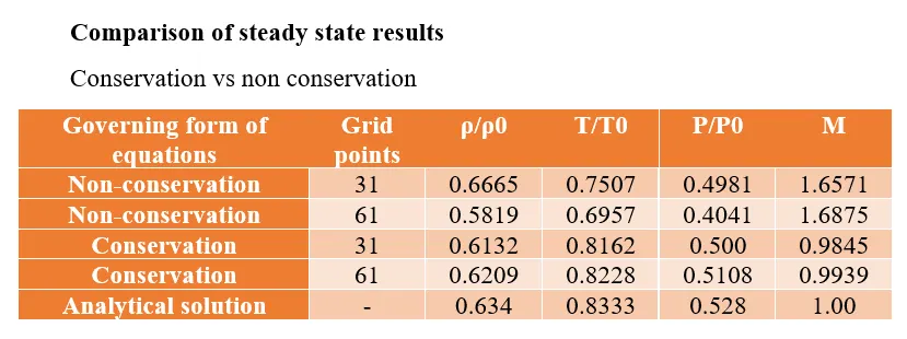
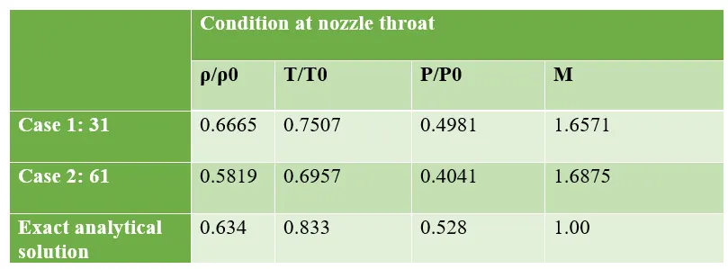
- The grid dependency test shows more robust and tolerant data close to analytical solution.
- At the end of time steps both conservation and non-conservation reaches steady state conditions.
- Computing the algorithm for non-conservation is much simpler than conservation form.
- In case of same grid points the non-conservation yields more accurate and better results for primitive variables like density, temperature, pressure and Mach no approximately close to analytical conditions.