Exploring the GUI and Modeling of Intercooler by GT-POWER
To explore the GUI settings of GT power
GT suite or GT power is a powerful 1D system simulation modelling and system calibration software, which uses multi physics tool to solve problems related to thermal, fluid, structure, aerospace system, engine modelling and thermal management systems.
Modules of GT Power:
3D Quick references: This tool provides a complete glance of controlling commands like modelling function, dimensioning, general command, project command, selection mode, slicing command.
Cool 3D: It is a tool used to build 3D models of thermal management flow systems with option discretized and later used in GT suite.
DOE post: Design of experiment used to
- Identify the design variables
- Identify optimal values
- Meet design objectives
Gem 3D: It is a tool used to build 3D models to build flow, thermal and mechanical systems that can be discretized and transform into model files for use with GT suite.
GT ISE: This is an interface of GT to build models and simulation. It creates the model in sequential orientation step by step like engine cylinder, engine crankshaft, cyl pipe, combustion, valve train, cooling, lubrication etc.
GT POST: It is a powerful data analysis tool used to plot views and manipulate data either by GT simulation or external source. Also plotting of graph and viewing animation effects can be studied.
VT design: Interactive cam/ valve train supplied with GT suite that can be used as a preprocessor. VT design composed of cam design, valve train design and spring design features.
GT space-claim: This tool is used to import CAD models of various format, extract volumes and can export them in discretization in GEM 3D.
Optimization: It is a build in module which is used for model optimization according to user specific condition.
GT suite is tailor made to provide different domains of industrial application as shown below.
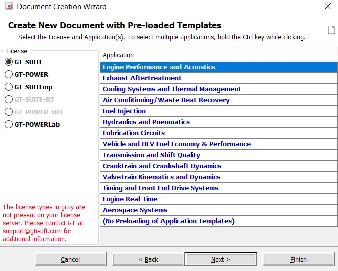
Engine performance and acoustics
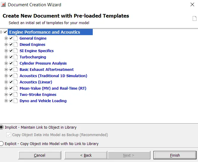
Exhaust after treatment
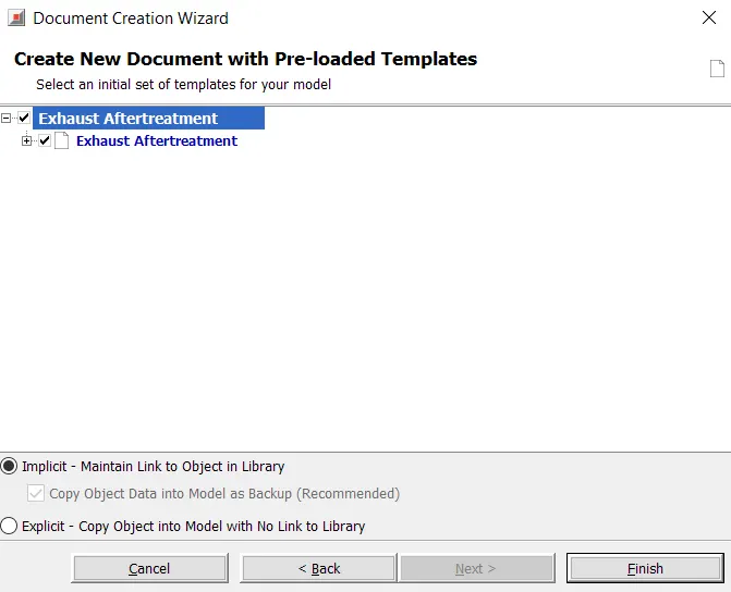
Cooling system and thermal management
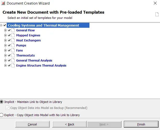
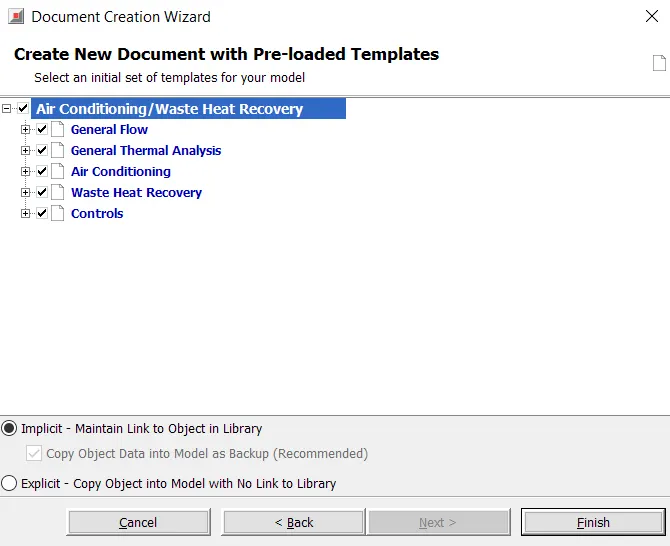
Air conditioning and waste heat recovery
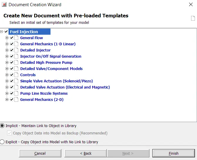
Fuel injection
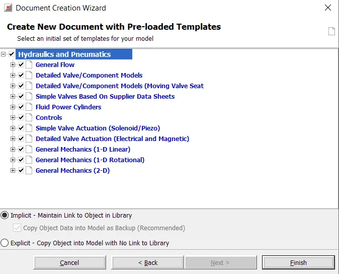
Hydraulics and Pneumatics
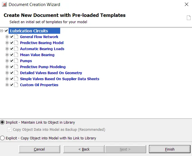
Lubrication circuit
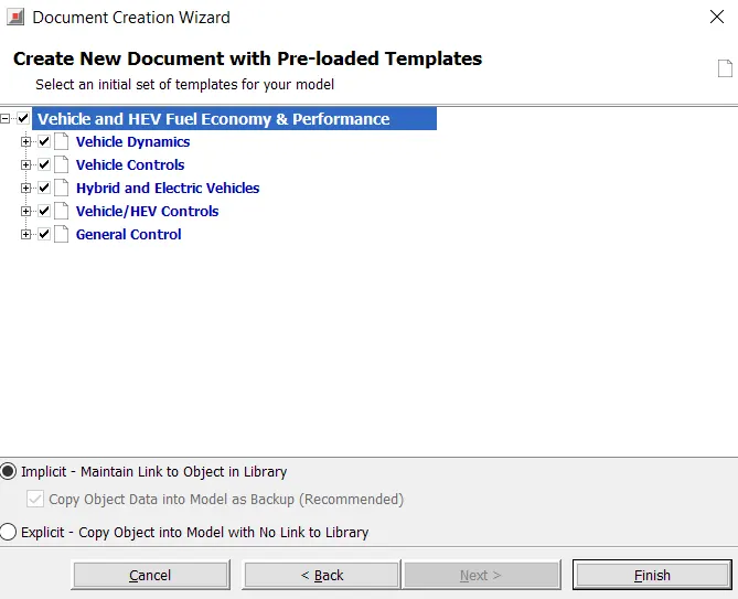
Vehicle and HEV fuel economy
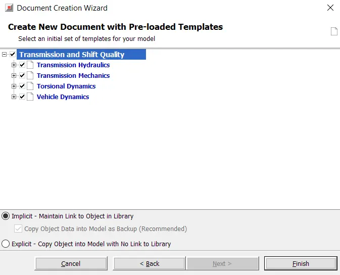
Transmission and shift quality
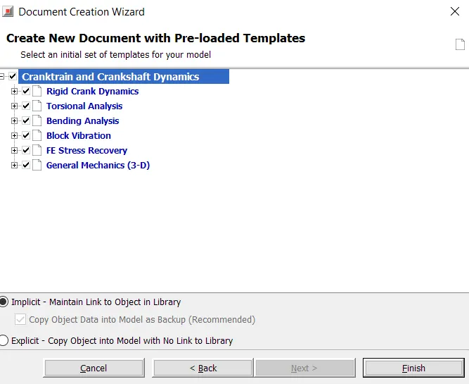
Crank train and crank shaft dynamics
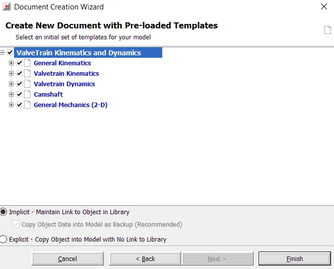
Valve train kinematics and dynamics
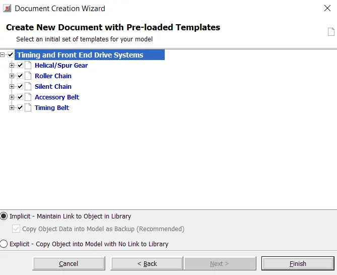
Timing and front-end drive system
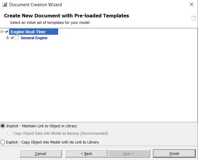
Engine real time
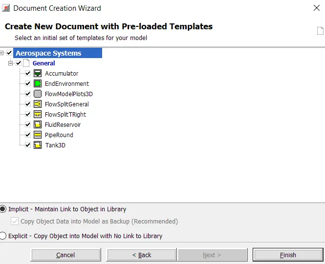
Aerospace systems
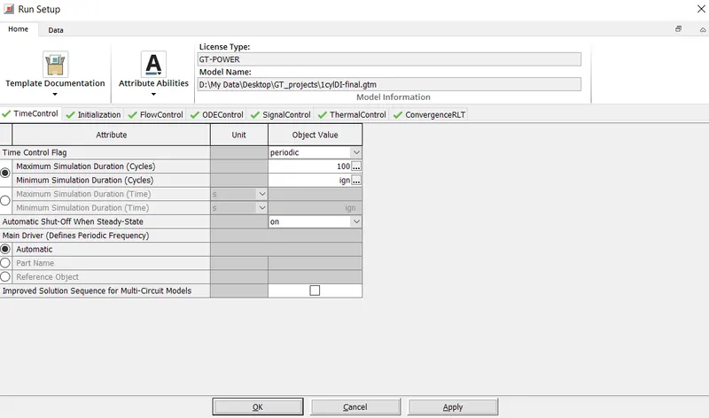
Locate following settings:
- Time control flag
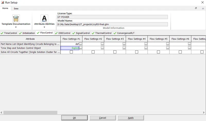
- Time step and solution control
- Integrator/Solver type
Time control flag
Defines the global simulation type with regard to time. One of the following options:
Periodic indicates that the model contains at least one circuit which contains a periodic event (i.e. engine cylinder “cycle”) and therefore requires tracking of results with respect to angle over each cycle. Any model that includes an ' EngineCrankTrain', ' CrankAnalysis' , or ' EngineCrankShaft' part should use the periodic option. Note that the simulation duration for a periodic simulation can be specified in cycles or in time, whichever is most convenient.
Continuous indicates that the simulation includes no periodic event, and therefore has no need to track results with respect to a cyclic angle. This is the typical setting for models that contain only quasi-steady fluid circuits such as coolant or underhood air. The simulation duration for a continuous simulation is typically specified in time.
Time step and solution control
Defines whether the circuit(s) in the column are periodic or continuous, potentially overriding the setting in the TimeControl folder. Different modules like ‘FlowControlExplicit', ' FlowControlImplicit', or ' FlowControlQS' reference object that can be used to define the numerical parameters for the explicit, implicit, or quasi-steady flow solver, respectively.
Integrator and solver type
Integrator/solver type used in the time-marching of all ODEs including mechanical, electrical and magnetic libraries.
Explicit-Adams-PECE Explicit Adams-Bashforth-Moulton predictor-corrector integration scheme with variable order accuracy. This integrator is recommended for large non-stiff problems, problems with a high maximum time step which have different scales and real time applications. It requires a tuning process in order to optimize its functionality.
Explicit-Runge-Kutta Explicit Runge-Kutta integration scheme that is 5 th order accurate. This integrator is recommended for non-stiff problems.
Implicit-Trapezoidal Implicit Trapezoidal integration scheme that is 2 nd order accurate. This integrator is recommended for moderately stiff problems.
Implicit-H.H.T. Implicit Hilber-Hughes-Taylor integration scheme that is 2 nd order accurate. This integrator is recommended for moderately stiff problems.
Implicit-Radau2 Implicit 2-stage Radau integration scheme that is 3 rd order accurate. This integrator is recommended for stiff problems.
Implicit-Radau3 Implicit 3-stage Radau integration scheme that is 5 th order accurate. This integrator is recommended for stiff problems.
Implicit-S.D.C.3 Implicit 3-stage Spectral Deferred Correction (S.D.C.) integration scheme that is 5 th order accurate. This integrator is recommended for very stiff problems.
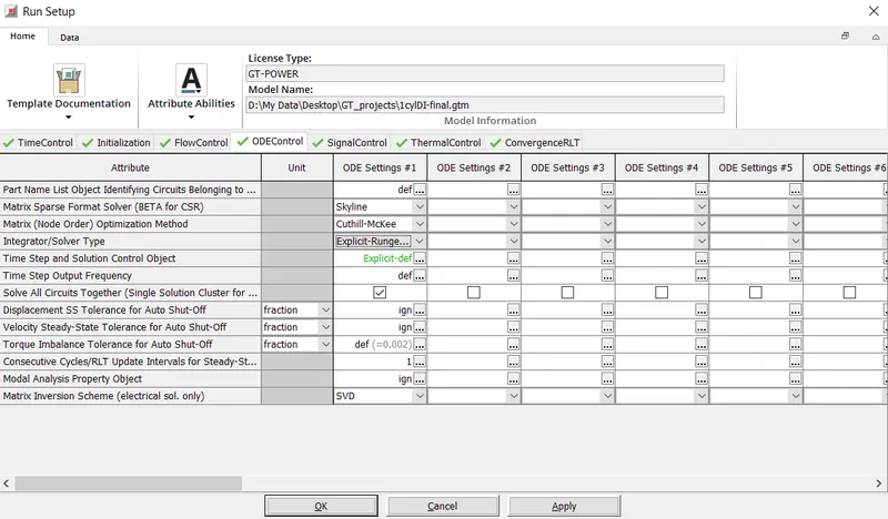
Explore intercooler tutorial and note down all settings of:
- Run setup
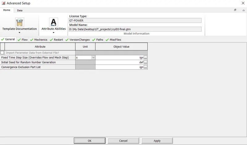
- Advanced setup
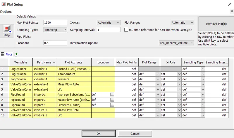
- Plot setup
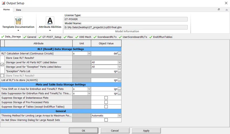
- Output setup
Run setup
Advanced setup
Plot setup
Output setup
Problem:
Given
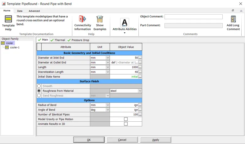
- Diameter of cooler inlet and outlet pipe= 50 mm
- Length of the CAC= 1000 mm
- Inlet mass flow rate = 1200 kg/ h at 100 degC
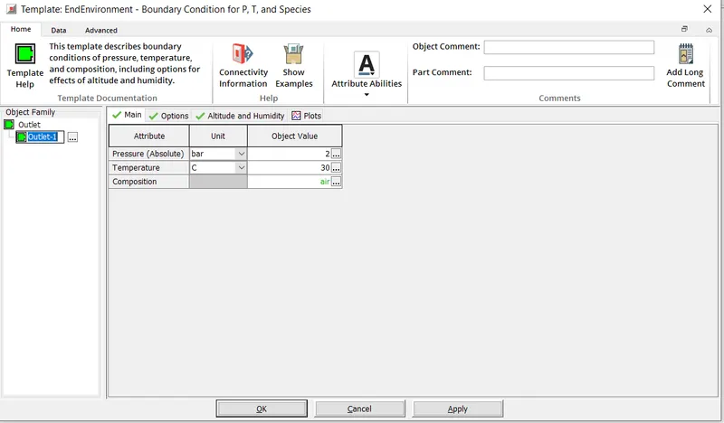
- Outlet pressure 2 bar at 30 deg C
- Calculate the total heat transfer at Charge air cooler (CAC)
- Calculate pressure drop across CAC
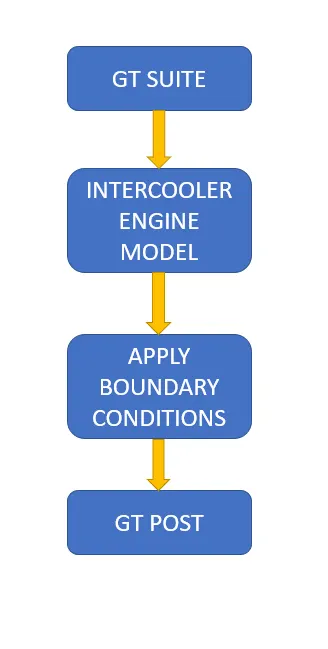
Modelling approach:
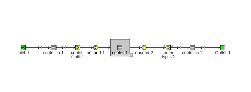
Simulation model:
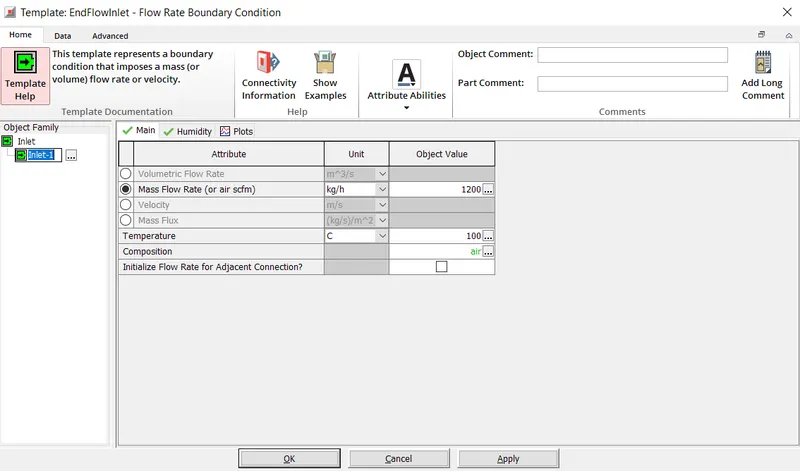
Boundary conditions:
Inlet mass flow rate = 1200 kg/ h at 100 degC
Diameter of cooler inlet and outlet pipe= 50 mm
Length of the CAC= 1000 mm
Outlet pressure 2 bar at 30 deg C
GT POST SIMULATION:
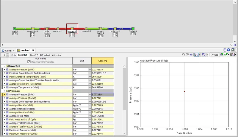
Pressure variation across the inlet and outlet section of intercooler
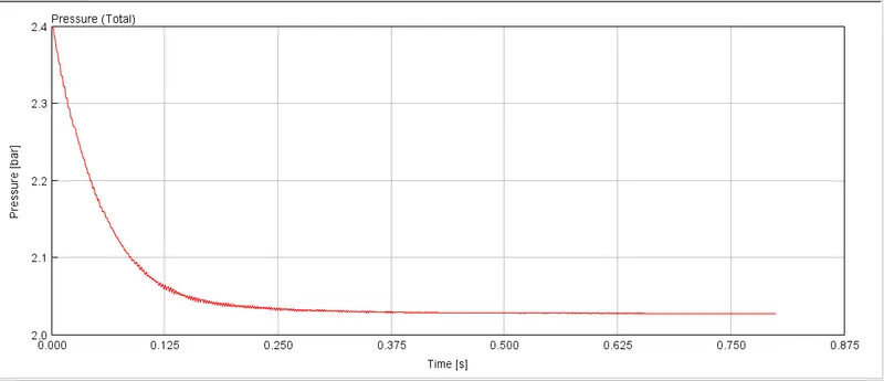
Pressure variation with respect to time
Pressure drop across the intercooler= 1.099Pa
Temperature variation across the inlet and outlet section of intercooler
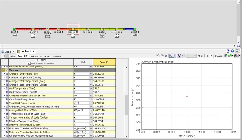
Temperature variation with respect to time
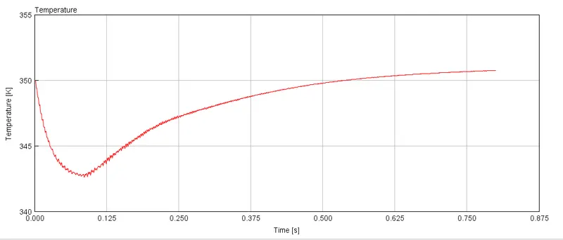
Inlet temperature= 370K
Outlet temperature= 350K
Total heat transfer area= 15.70m2
Average heat transfer coefficient at inlet= 125.83 W/m2K
Average heat transfer coefficient at outlet= 119.20 W/m2K
Total heat transfer at inlet= `h A triangleT=125.83*15.70*20=39510.62W`
Total heat transfer at inlet= `h A triangleT=119.20*15.70*20=37428.8W`
Conclusions:
- The GT suite GUI format has been explored.
- For the intercooler engine, heat transfer rate and pressure drop across the CAC has been computed.