Conjugate heat transfer analysis of Exhaust Port using Ansys fluent

Abstract:

Conjugate heat transfer analysis plays an important role in predicting the thermal performances and effectively capture the boundary effect. In this case study an exhaust manifold is analyzed using CHT approach to predict the heat transfer coefficient value at the interface of the boundary wall of two different domain. Using k-omega turbulent model the capture of boundary effect is taken accurately and also the factors that account for better HTC prediction.

Theory:

Conjugate heat transfer allows simulation of heat transfer between solid and fluid domain by exchanging thermal energies at the interface between them. Some typical turbulence model is used in modelling CHT are laminar, RANS, LES. In solids conduction often dominates and in fluids, convection usually dominates. Efficiently combining heat transfer in solid and fluid is the key to design effective coolers, heaters and heat exchangers. Heat transfer in solid and fluid are combined in a majority of application. Typical application of CHT can be performed to improve cooling performance of water jacket and increase engine life. Advancements in cooling for application in gas turbine to understand the complex heat transfer interactions. Critical cooling application involves internal and external film cooling. CHT analysis provides thermal distribution in solid and coolant of engine to provide better insight in velocity distribution and designing thermal load capacity.

Heat Transfer by Solids and Fluids

Heat Transfer in a Solid

In most cases, heat transfer in solids, if only due to conduction, is described by Fourier’s law defining the conductive heat flux, q, proportional to the temperature gradient: .

For a time-dependent problem, the temperature field in an immobile solid verifies the following form of the heat equation:

Heat Transfer in a Fluid

Due to the fluid motion, three contributions to the heat equation are included:

1. The transport of fluid implies energy transport too, which appears in the heat equation as the convective contribution. Depending on the thermal properties on the fluid and on the flow regime, either the convective or the conductive heat transfer can dominate.
2. The viscous effects of the fluid flow produce fluid heating. This term is often neglected, nevertheless, its contribution is noticeable for fast flow in viscous fluids.
3. As soon as a fluid density is temperature-dependent, a pressure work term contributes to the heat equation. This accounts for the well-known effect that, for example, compressing air produces heat.

Conjugate Heat Transfer Applications

Effective Heat Transfer

Efficiently combining heat transfer in fluids and solids is the key to designing effective coolers, heaters, or heat exchangers.

The fluid usually plays the role of energy carrier on large distances. Forced convection is the most common way to achieve high heat transfer rate. In some applications, the performances are further improved by combining convection with phase change (for example liquid water to vapor phase change).

Even so, solids are also needed, in particular to separate fluids in a heat exchanger so that fluids exchange energy without being mixed.

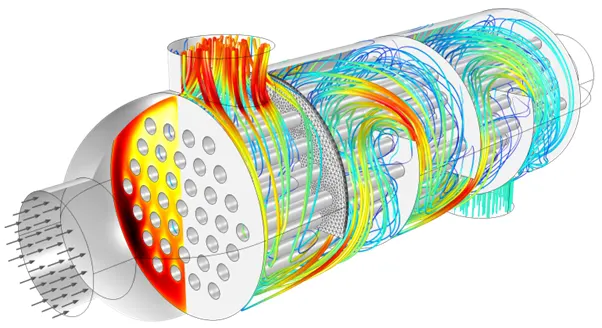
Flow and temperature field in a shell-and-tube heat exchanger illustrating heat transfer between two fluids separated by the thin metallic wall.

Heat sinks are usually made of metal with high thermal conductivity (e.g. copper or aluminum). They dissipate heat by increasing the exchange area between the solid part and the surrounding fluid.

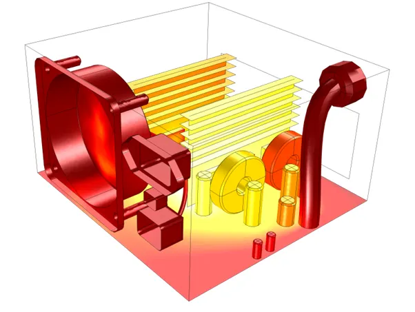
Energy Savings

Heat transfer in fluids and solids can also be combined to minimize heat losses in various devices. Because most gases (especially at low pressure) have small thermal conductivities, they can be used as thermal insulators… provided they are not in motion. In many situations, gas is preferred to other material due to its low weight. In any case, it is important to limit the heat transfer by convection, in particular by reducing the natural convection effects. Judicious positioning of walls and use of small cavities helps to control the natural convection. Applied at the micro scale, the principle leads to the insulation foam concept where tiny cavities of air (bubbles) are trapped in the foam material (e.g. polyurethane), which combines high insulation performances with light weight.

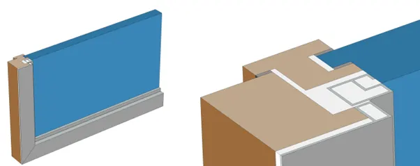
Window cross section (left) and zoom-in on the window frame (right).

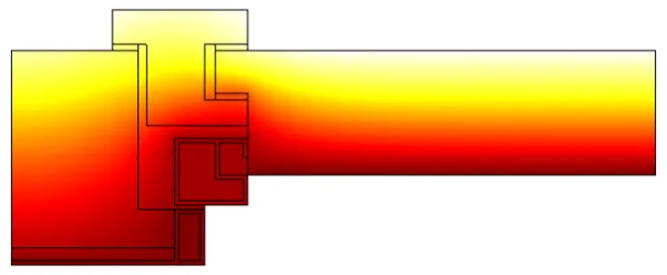
Temperature profile in a window frame and glazing cross section from ISO 10077-2:2012 (thermal performance of windows).

Fluid and Solid Interactions

Fluid/Solid Interface

The temperature field and the heat flux are continuous at the fluid/solid interface. However, the temperature field can rapidly vary in a fluid in motion: close to the solid, the fluid temperature is close to the solid temperature, and far from the interface, the fluid temperature is close to the inlet or ambient fluid temperature. The distance where the fluid temperature varies from the solid temperature to the fluid bulk temperature is called the thermal boundary layer. The thermal boundary layer size and the momentum boundary layer relative size is reflected by the Prandtl number : for the Prandtl number to equal 1, thermal and momentum boundary layer thicknesses need to be the same. A thicker momentum layer would result in a Prandtl number larger than 1. Conversely, a Prandtl number smaller than 1 would indicate that the momentum boundary layer is thinner than the thermal boundary layer. The Prandtl number for air at atmospheric pressure and at 20°C is 0.7. That is because for air, the momentum and thermal boundary layer have similar size, while the momentum boundary layer is slightly thinner than the thermal boundary layer. For water at 20°C, the Prandtl number is about 7. So, in water, the temperature changes close to a wall are sharper than the velocity change.

The fluid flow and heat transfer problems can be tightly coupled through the convection term in the energy equation and when physical properties are temperature dependent. While analytical solutions exist for some simple problems, we must rely on computational methods to solve most industrially relevant applications.

CHT can be performed to improve cooling performance of the water jacket and increase engine life. Advancements in cooling for applications such as gas turbines components require improved understanding of the complex heat transfer mechanisms and the interactions between those mechanisms, which our engineers can perform without hassle. Critical cooling applications often rely on multiple thermal protection techniques, including internal cooling, external film cooling, etc. which are efficiently used by our analysis to cool components and limit the use of coolant. We do extensive support for Motor and Battery CHT Analysis to get optimized design for High voltage systems. Conjugate Heat Transfer analysis provides the temperature distribution in solid and coolant of the engine and clear insight on velocity distribution and mechanism of heat transfer of coolant. Results of CHT analysis become input to structural simulations as thermal loads.

We have a wide experience in Engine CHT Analysis for various type of engines like Bikes, Passenger Cars, Racing cars, Commercial Vehicles, Marine, Agricultural equipment and Earth-moving equipment etc.

Problem statement:

1. Give a brief description of why and where a CHT analysis is used.
2. Maintain the y+ value according to the turbulence model and justify the results.
3. Calculate the wall/surface heat transfer coefficient on the internal solid surface & show the velocity & temperature contours in appropriate areas.
4. How would you verify if the HTC predictions from the simulations are right? On what factors does the accuracy of the prediction depend on?

Modelling approach

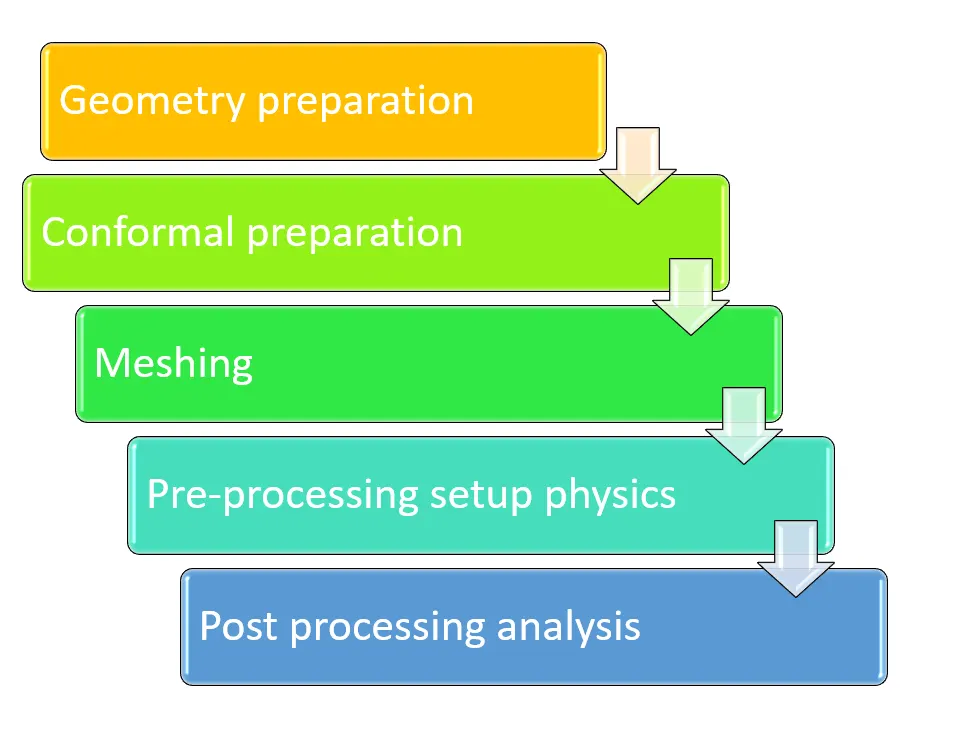
Geometry preparation:

• Import the geometry to the space claim from step file format.
• 
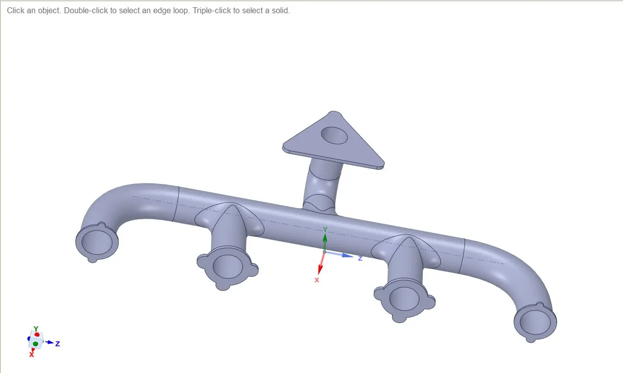
• Prepare the geometry for extracting the fluid volume from the solid domain. To do that go to prepare physics. Click on volume extraction.
• 
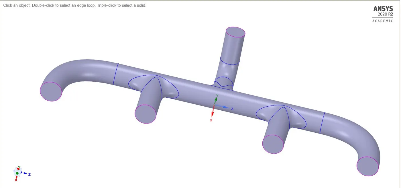
• Select the inlet edges and outlet edges of the exhaust port.
• Now move the solid and fluid domain to a new component.
• This is obtained by right click on the work tree diagram and select move to new component.
• Go to workbench, select share prep option. After the topological sharing will be completed, the entire internal region will be highlighted red. The external edges of inlet and outlet will appear as pink.
• 
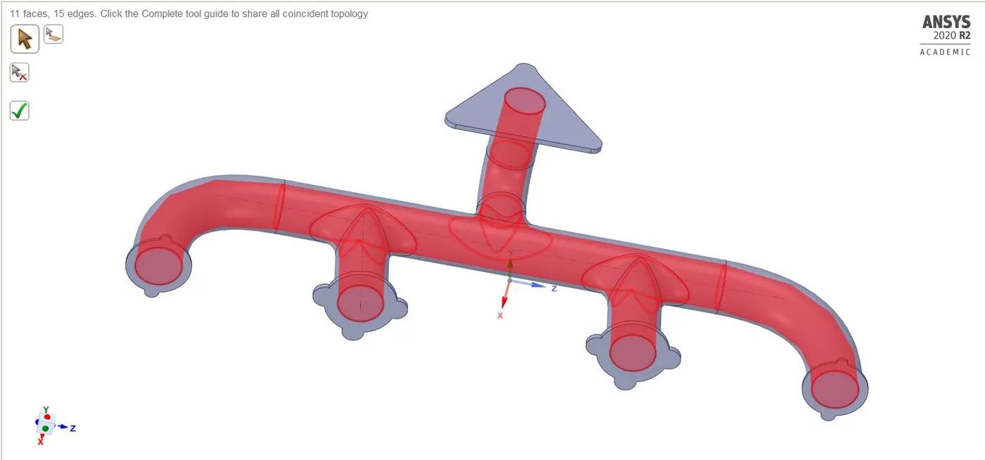
• Once topology, sharing is completed, the final geometry preparation is completed.

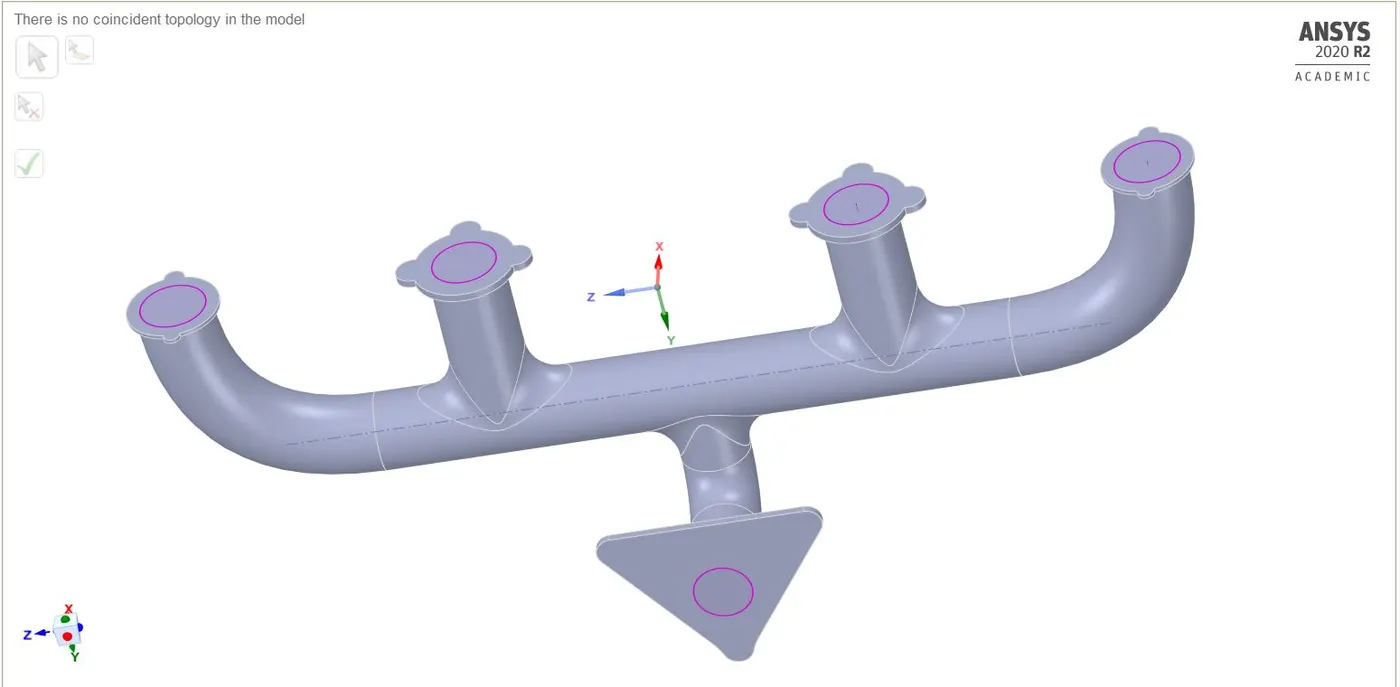
Conformal meshing is performed inorder to share the topology at the solid and fluid domain successfully. Without conformality the meshing interface would cuase a lot of interpoation at the boundaries which could eventually lead to improper meshing and non uniform heat conduction at the boundary zone. This may confirm about the smoothness in grading at the fluid domain due to the wall y+ effect.

Meshing:

• Open the meshing console.
• Once the geometry is opened, select mesh and click generate.
• A normal basic mesh will be created.
• 
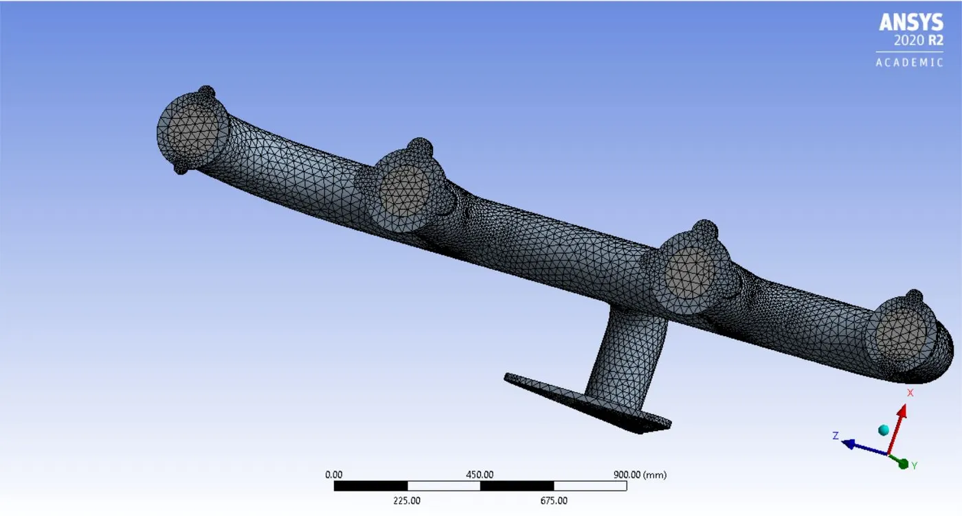
• Now refining the mesh.
• Before refining we create the named section to certain geometrical parts.
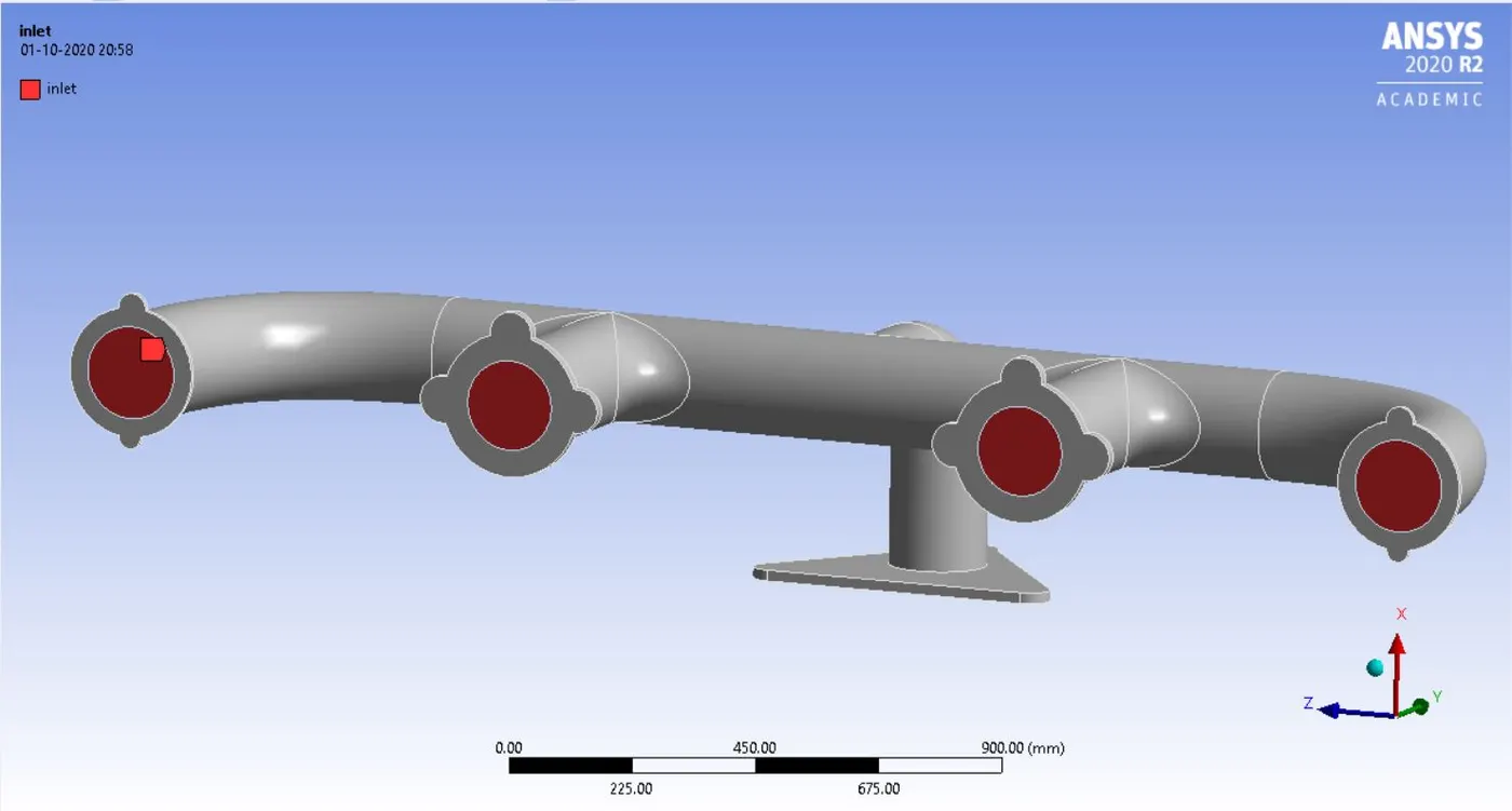
• Select the inlet faces of the exhaust port as inlet.
• 
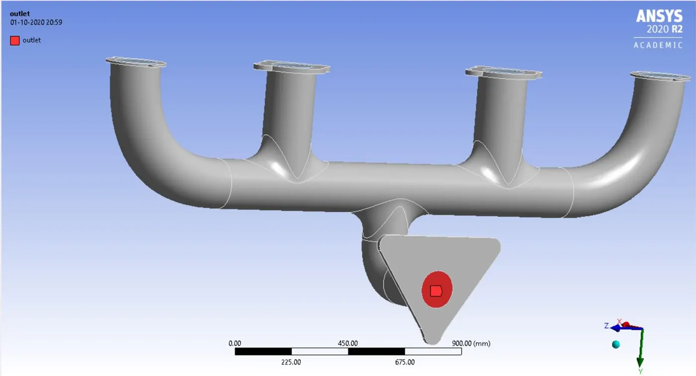
• Select the outer faces as outlet.
• 
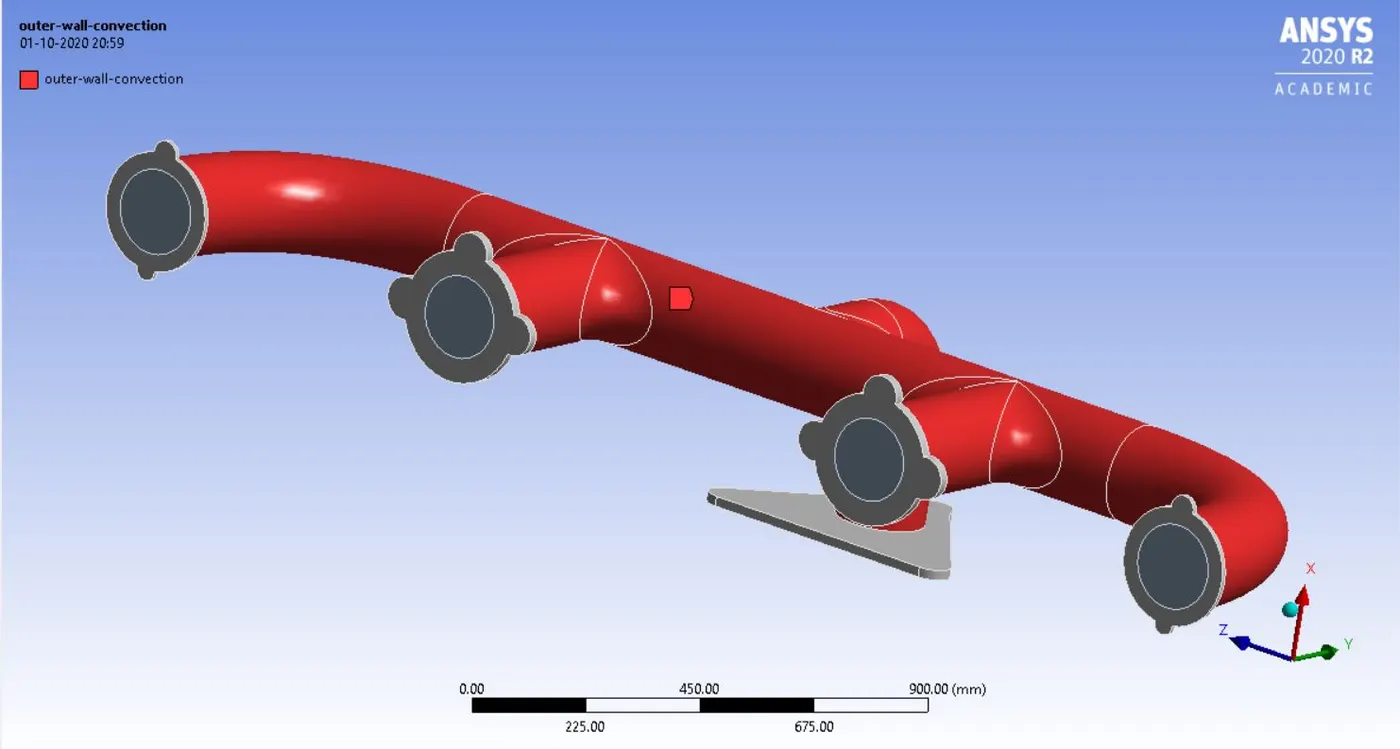
• Select the body of the exhaust port and define it as wall convective.
• 
• Select the inner fluid domain and name it as inflation layers.
• 
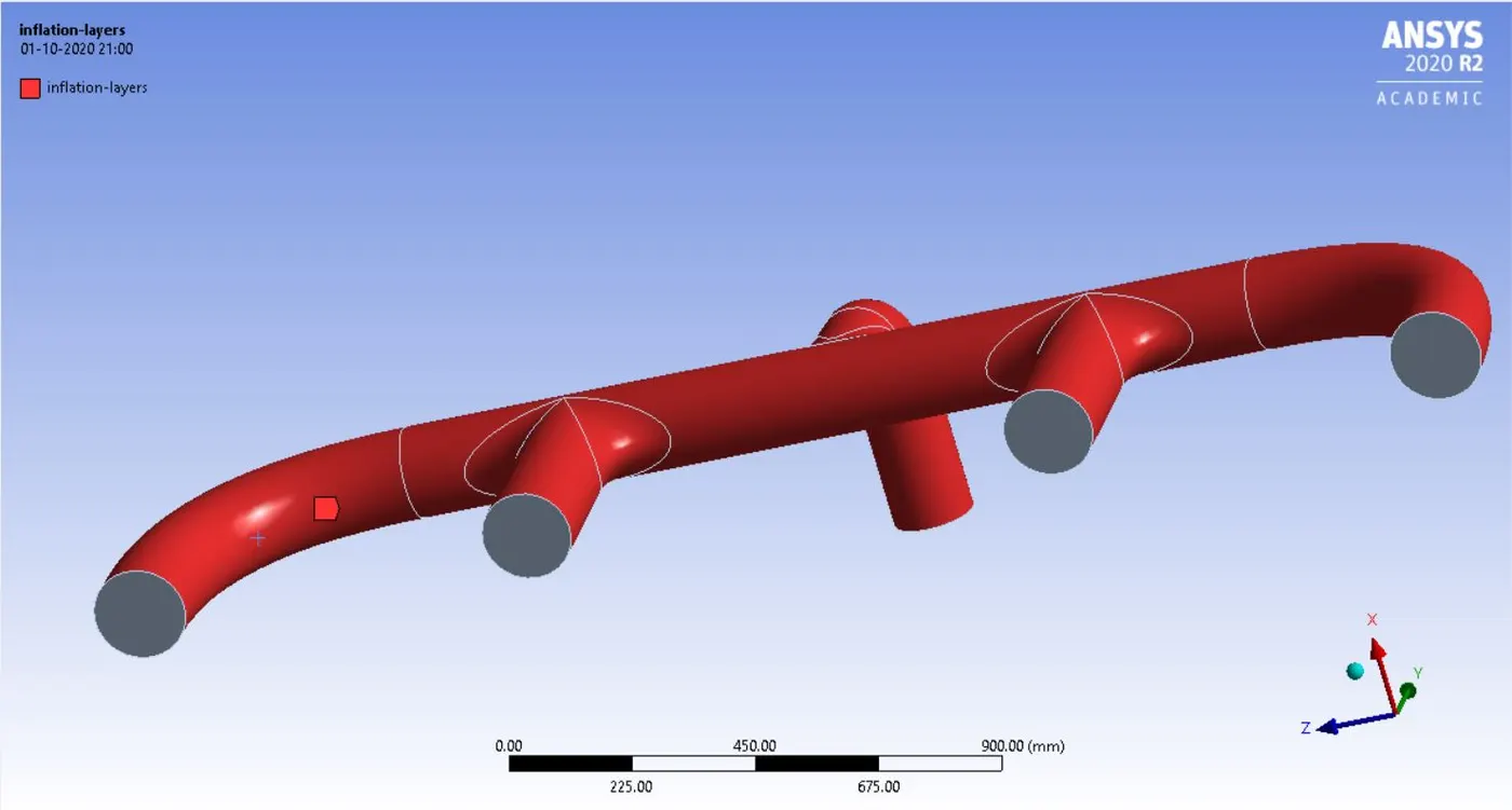
• Go to inflation properties and select chosen named selection as inflation layers.
• Give the appropriate no of layers according to y+ values and the corresponding total thickness.
• 
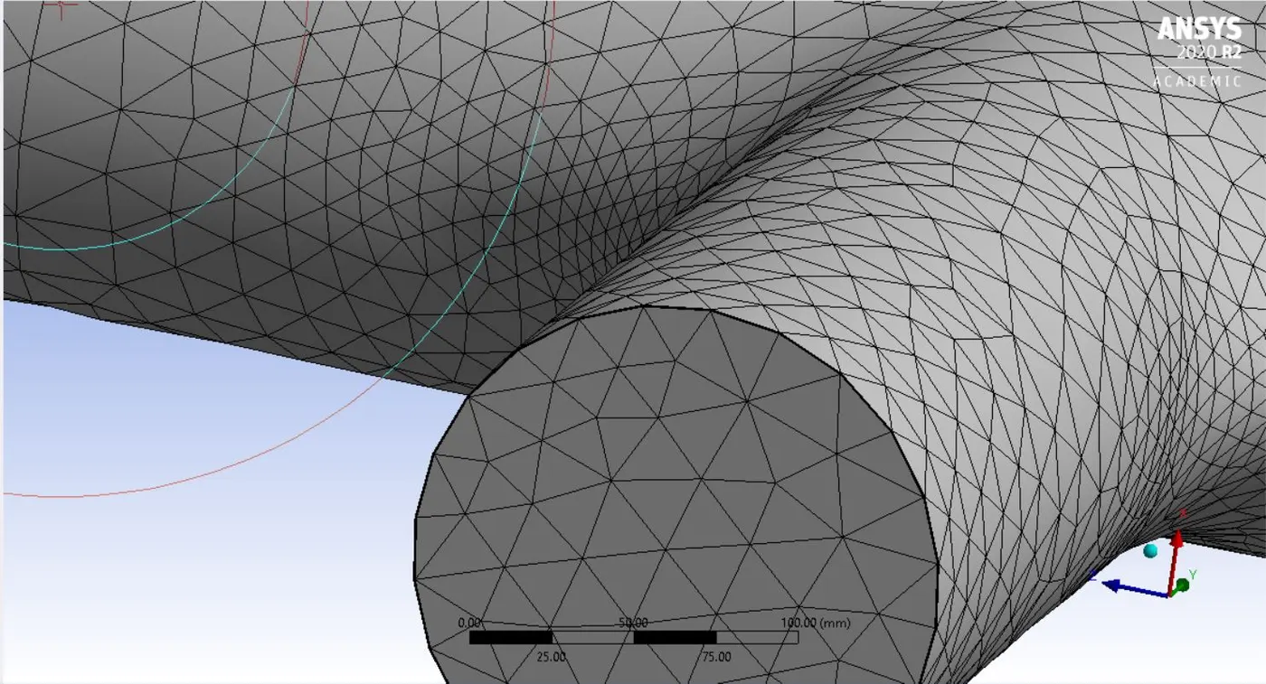
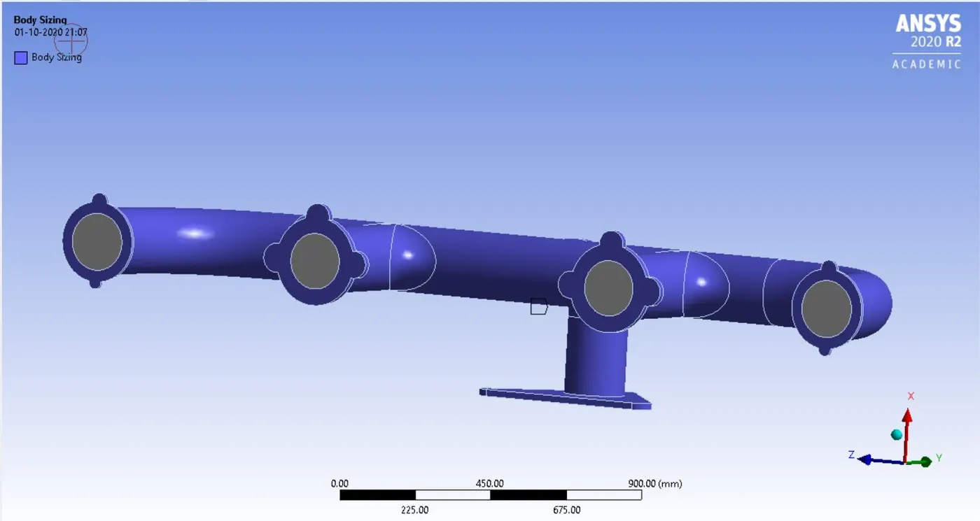
• Choose the sizing command and select the outer wall. Turn on the curvature capture mode.
• Give a desired value of mesh grading factor of 100mm.
• 

Setting up pre-processing physics:

• The first step is to choose the turbulent model, which in this case is k-omega model.
• 
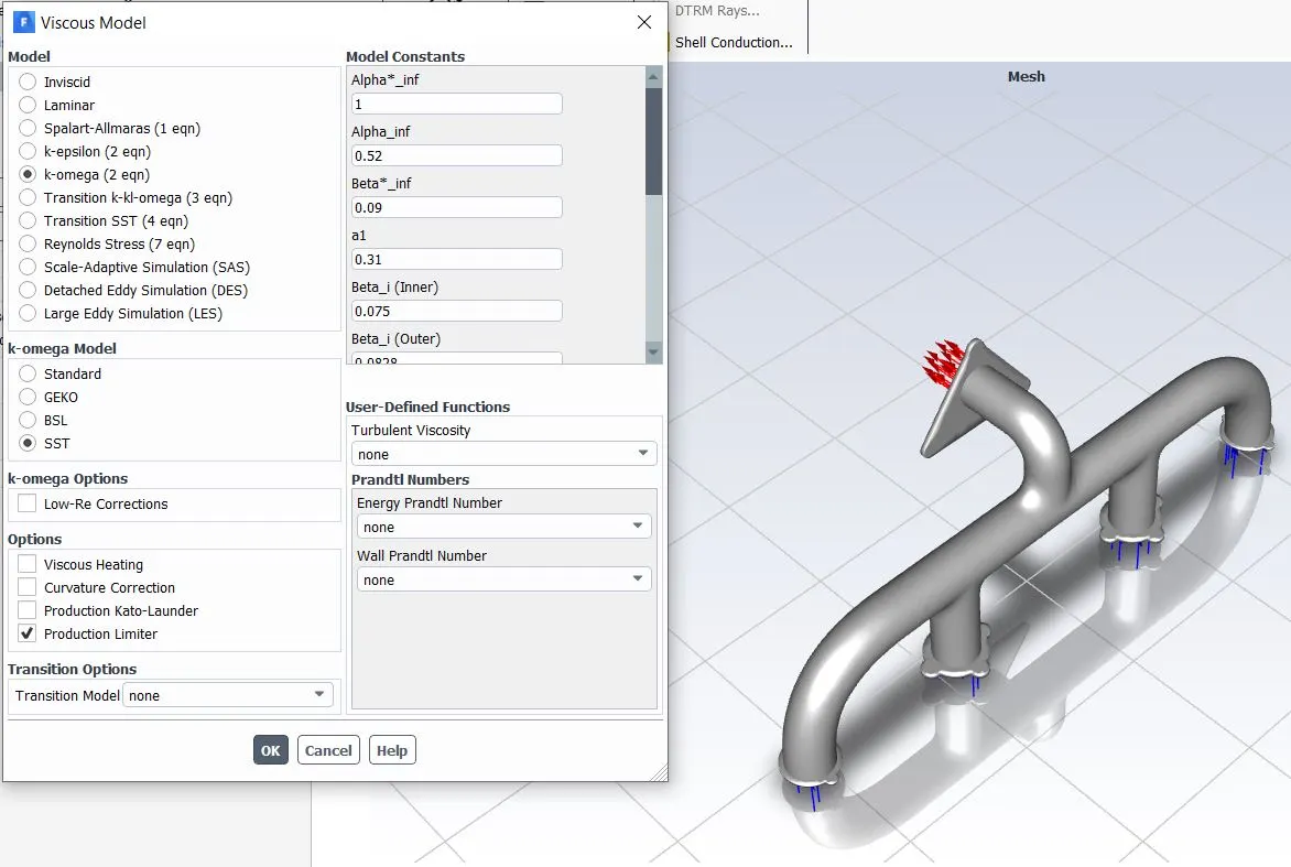
• In this problem, temperature of the inlet port is important so the temperature field is activated.
• The second step is to define the material, where fluid is taken as air and solid domain is taken as aluminum.
• Setting up the cell zone boundary conditions, we define the solid domain and fluid domain.
• Third step is to give the inlet of exhaust manifold as velocity of 5m/s and inlet temperature of 700k.
• 
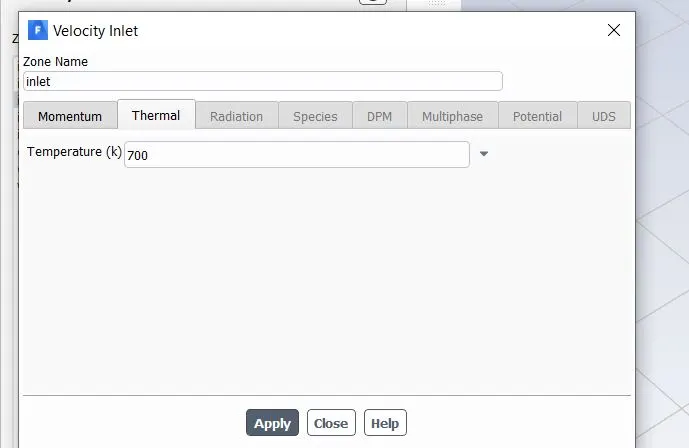
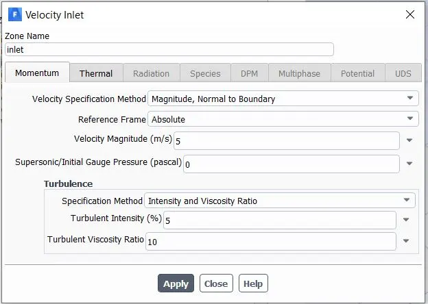
• The outlet is kept as pressure outlet and the outer wall convection is defined with a heat transfer coefficient of 20w/m2k. the other walls are kept as isothermal.
• 
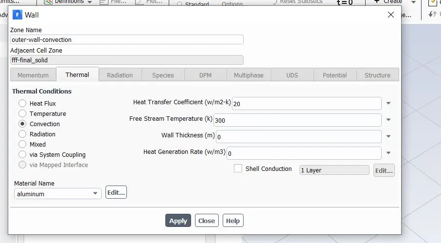
• Fourth step is to initialize the solution with hybrid initialization schemes.
• After initialization, we create a temperature contour at the zones of inlet, outlet, outer wall convection and other wall region.
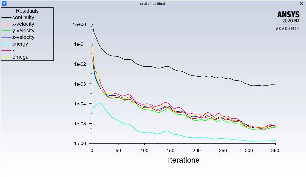
• Give the no of iterations to be performed and run the fluent solver.
• After convergence, check for the temperature contour zones.

Post processing physics simulation:

Baseline mesh setup

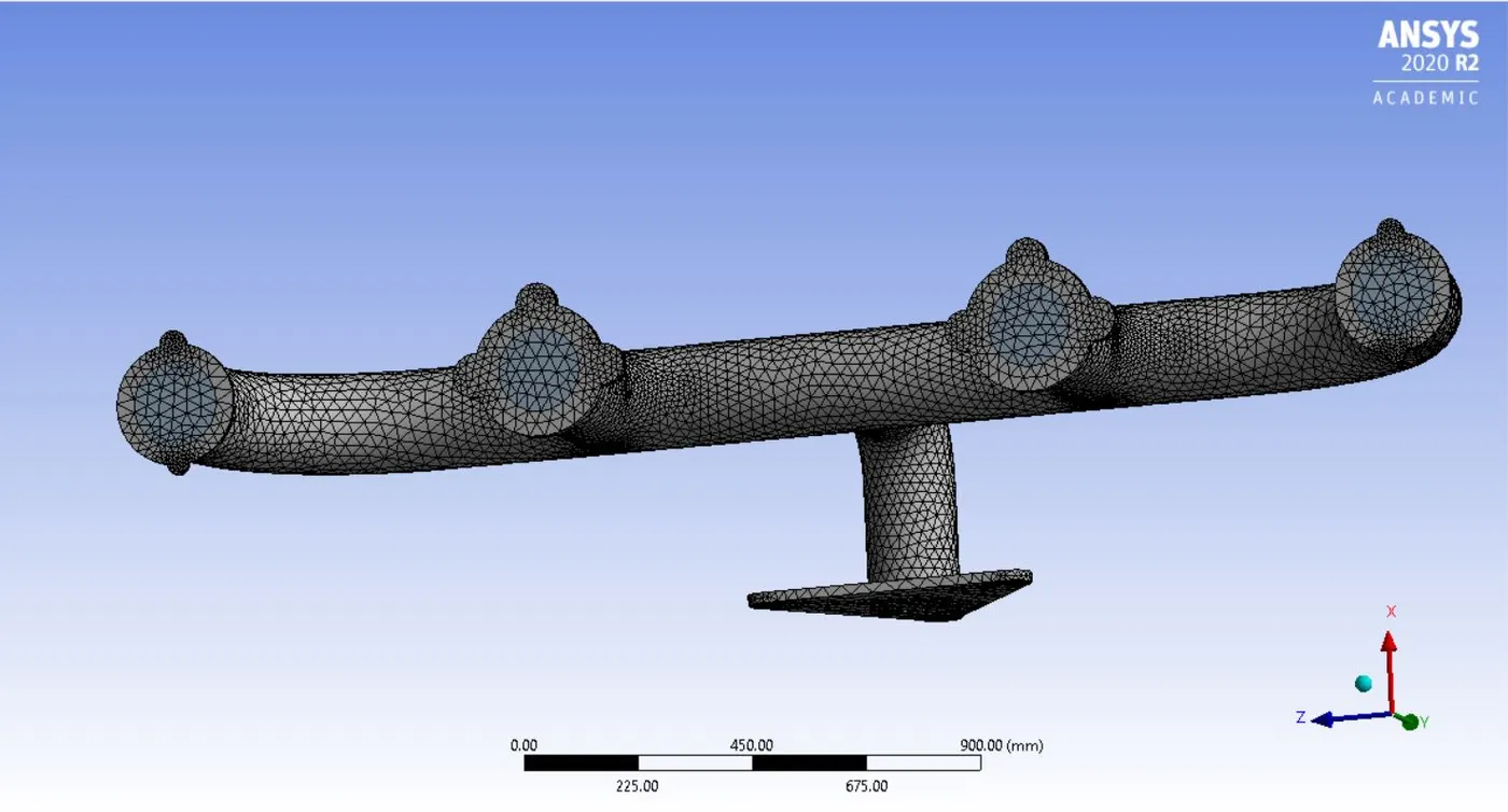
Nodes: 27451

Elements: 137651

Meshing zone

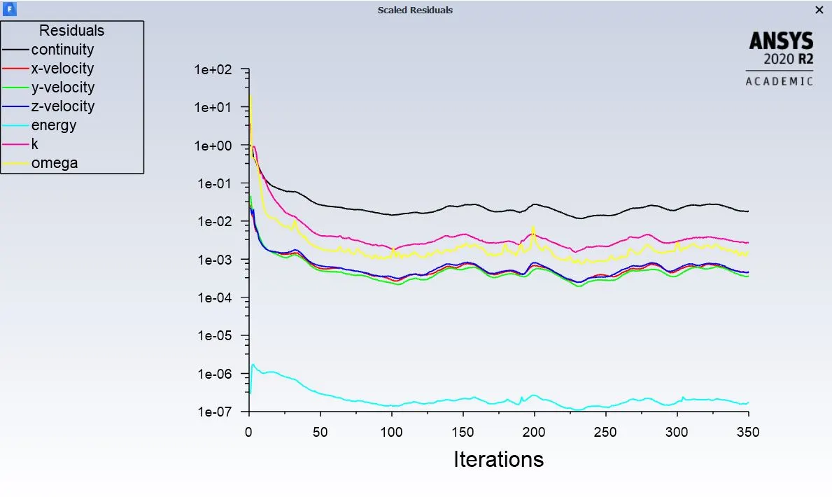
Convergence of iterations

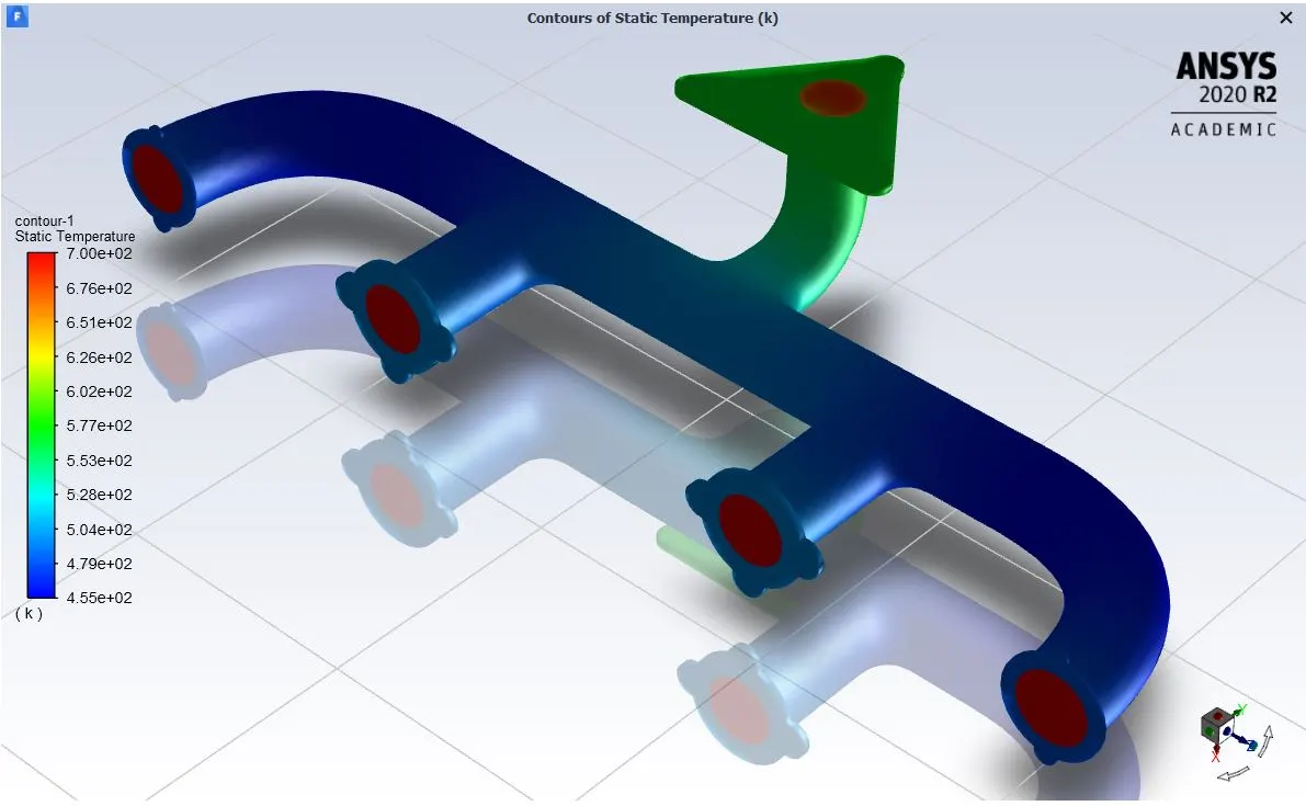
Temperature contour

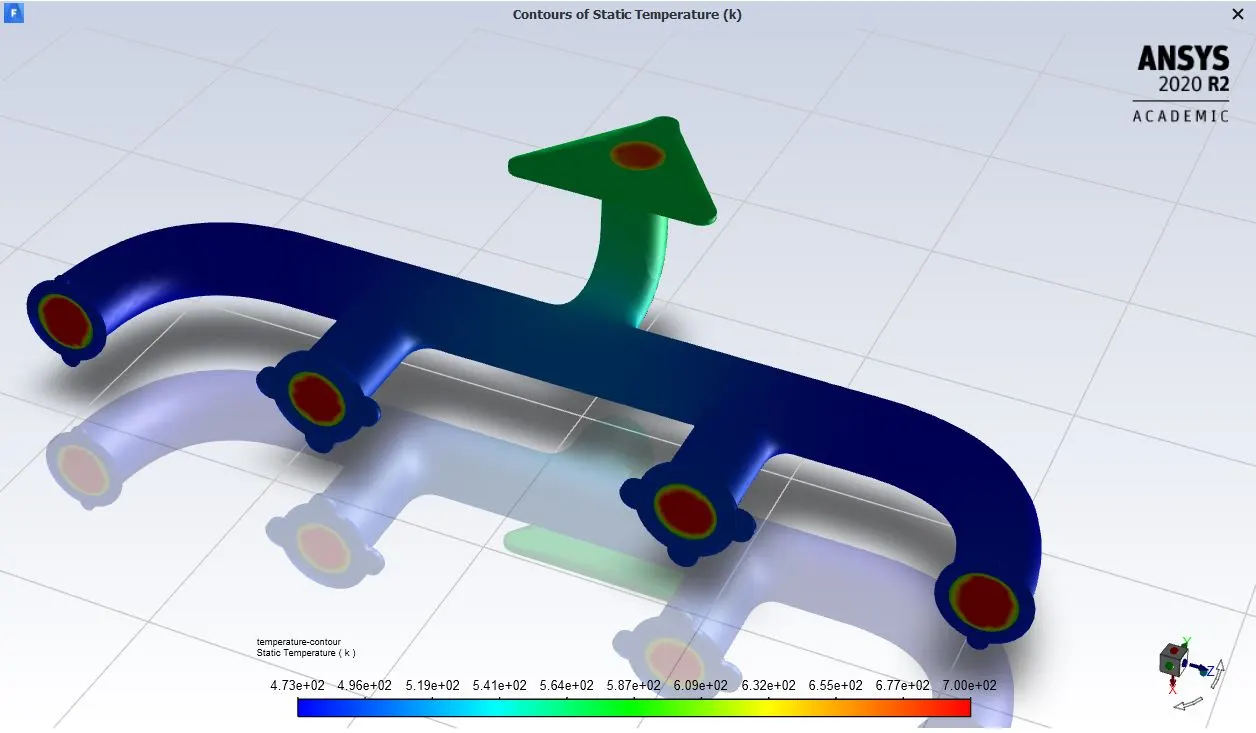
Temperature at the outer wall convection

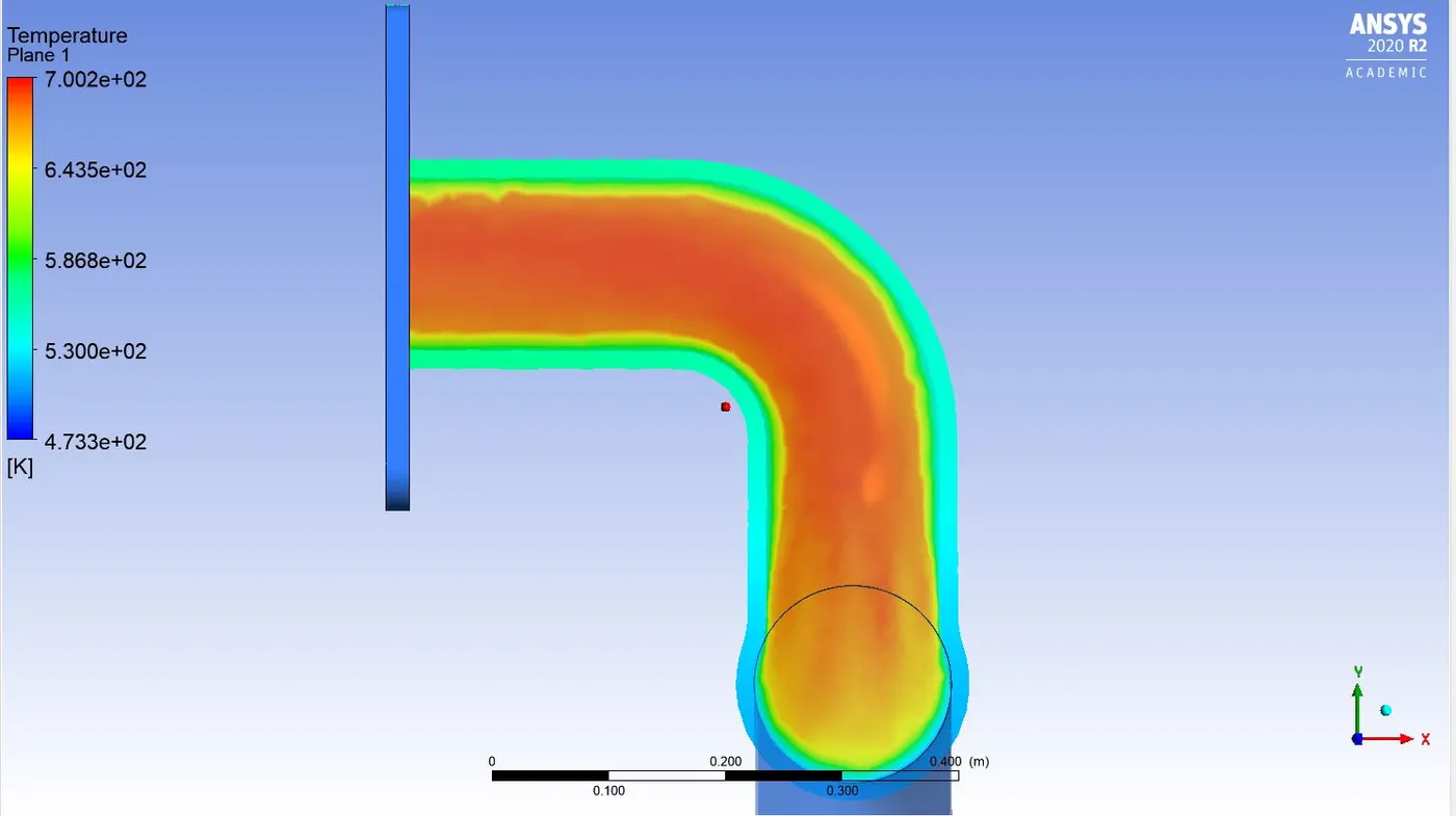
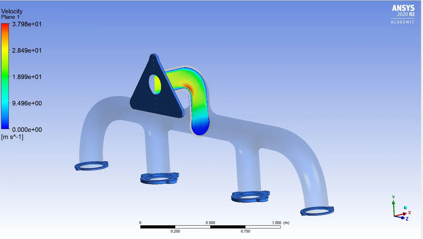
Velocity plane

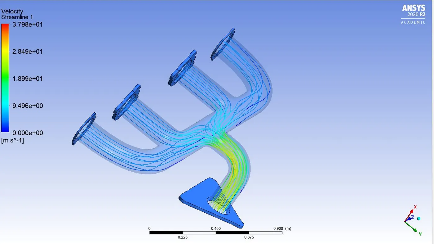
Velocity streamlines

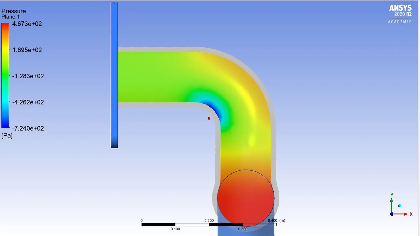
Pressure plane

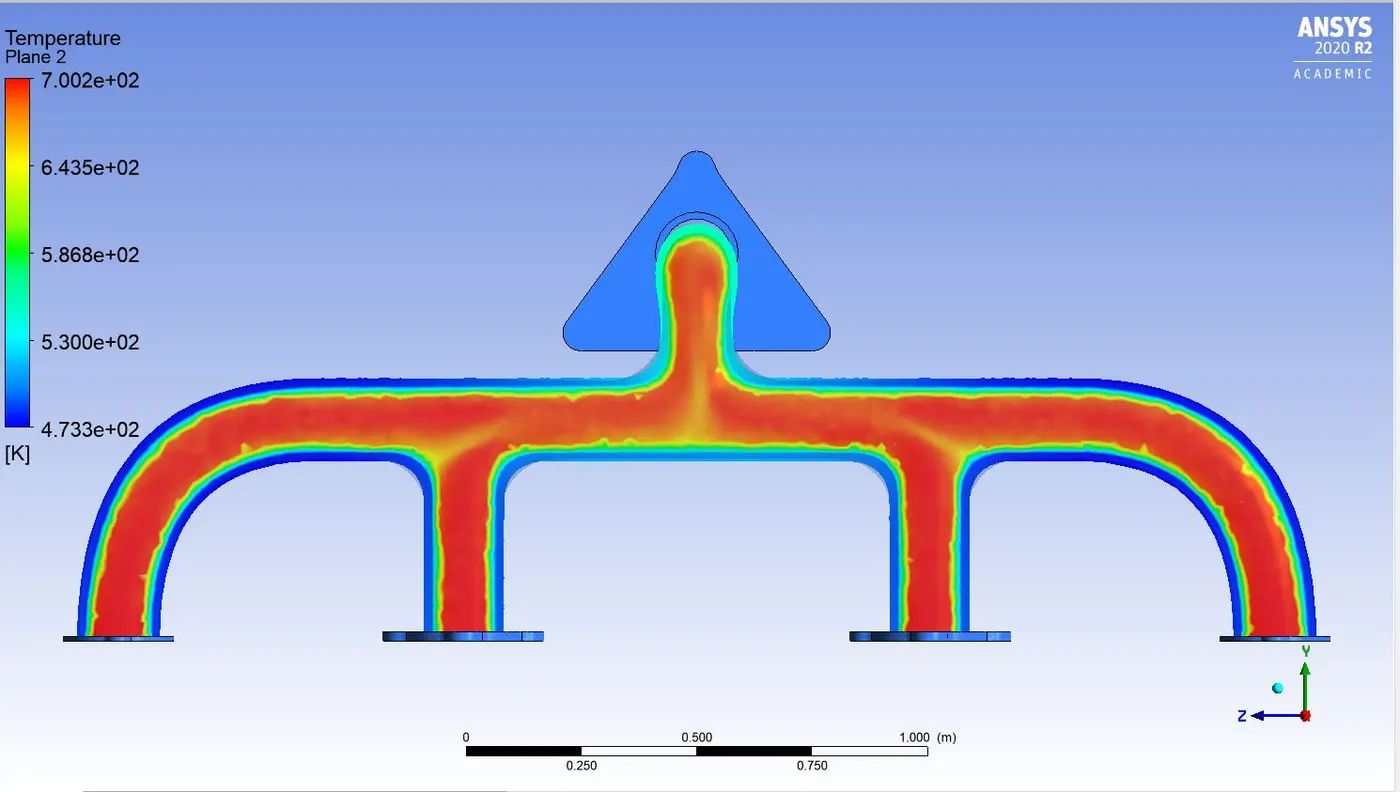
Temperature plane

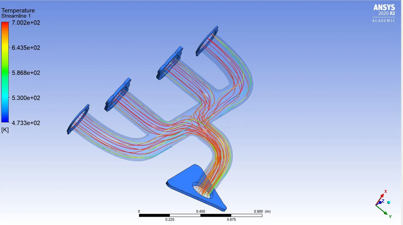
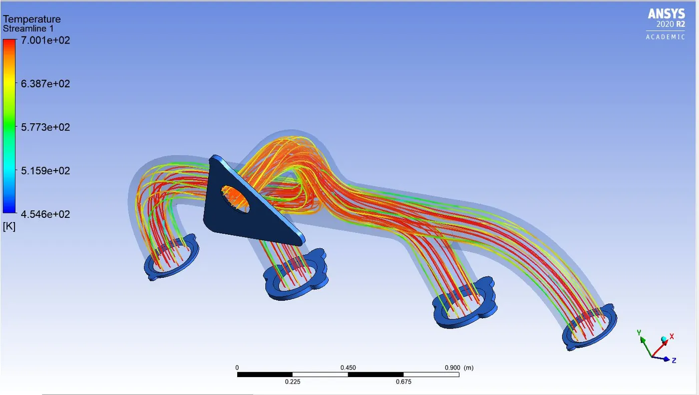
Temperature streamlines

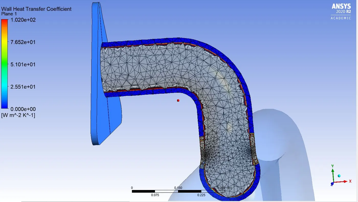
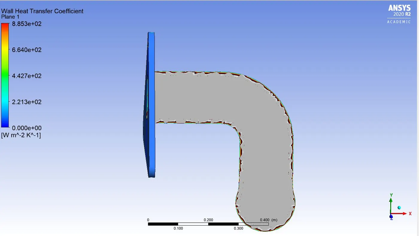
Predicted Heat transfer coefficient value at the wall boundary

Refined mesh setup

Nodes:87912

Elements:256337

Meshing zone

Convergence of iterations

Temperature contour

Wall y+ values

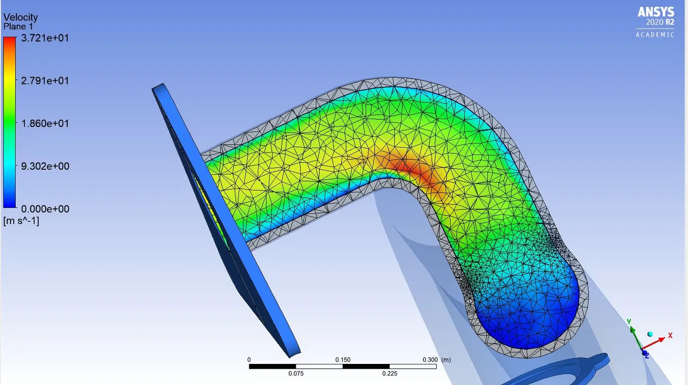
Velocity plane

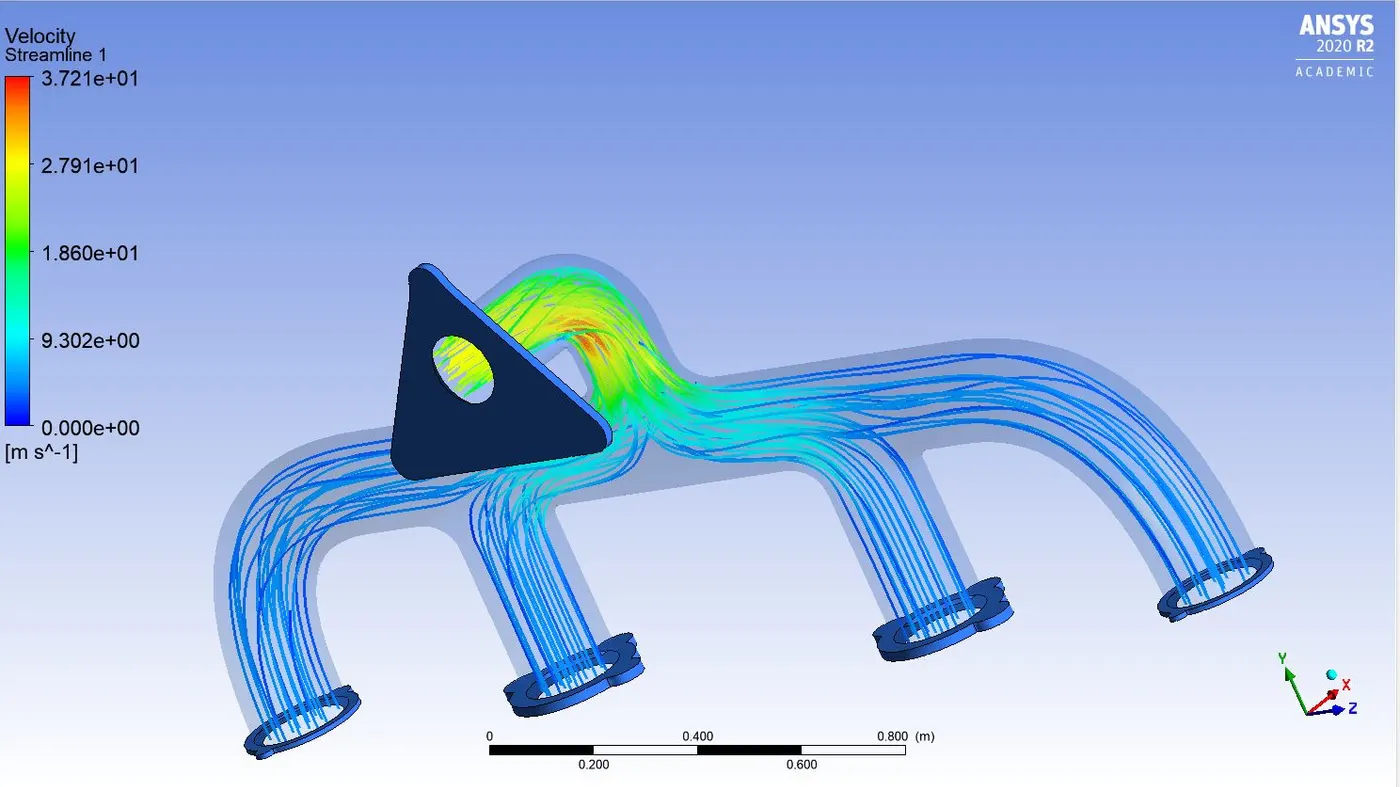
Velocity streamlines

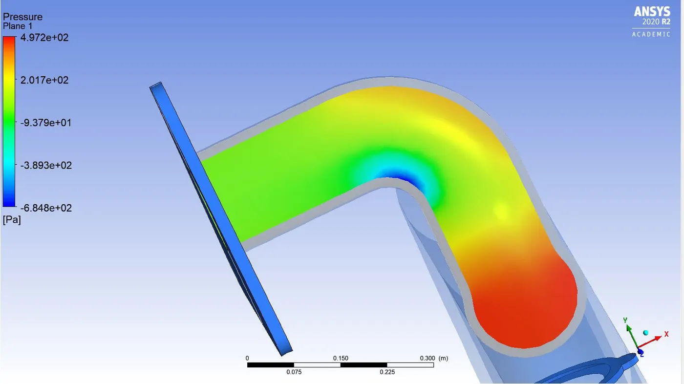
Pressure plane

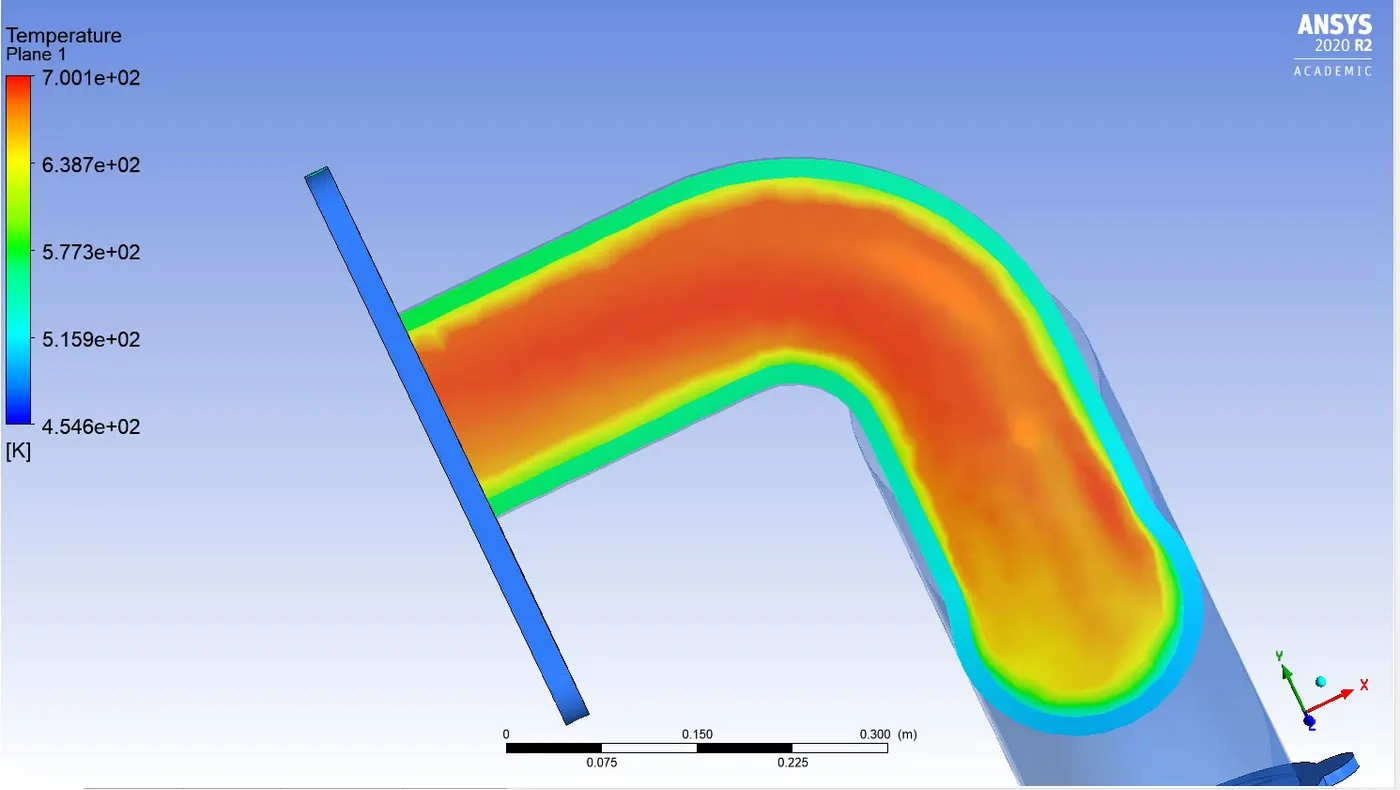
Temperature plane

Temperature streamlines

Predicted Heat transfer coefficient value at the wall boundary

Factors on which the prediction accuracy depends upon:

1. Correct choosing the value y+ which satisfies the turbulent model, by effectively capturing the velocity and temperature at the boundary wall interface.
2. Meshing at the junction of the solid and fluid domain. With a definite value of y+, the no of inflation layers and the growth rate determines the smooth flow of heat transfer between the two zones.
3. The heat transfer coefficient can be predicted by another factor called Nusselt no which is given by Nu=0.023*Re^(4/5)*Pr^n.
4. The experimental heat transfer value lies around 980 but the simulated value gave around 885, which is somewhat closer to it. It can be predicted more accurately with correct meshing and choosing correct y+ value.

Conclusions:

1. The conjugate heat transfer analysis is successfully performed in two cases viz baseline and refine setup.
2. The maximum velocity for baseline case is found to be m/s and for refined case the maximum velocity is found to be m/s.
3. The wall y+ value as predicted from the k-omega model lies accurately within the range 0-5.
4. For the refined case setup, the heat transfer coefficient values is found to be 885 at the junction between the fluid and the solid boundary wall.