Week 6 - Multivariate Newton Rhapson Solver
Theory:
In order to estimate the combustion process inside a combustion chamber, it is fundamental to evaluate the mole fractions of a gas which consists of burned mixtures. A set of combination equations must be solved to evaluate the mixture composition.
Newton Raphson approach:
The basic equation for newton Raphson is:
`x^(i+1)=x^i-(f(x^i )/(f^' (x^i ) ))`
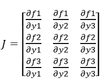
For a multivariate-systems, we convert all the variables in vector form and we represent it in the form
`X^(i+1)=X^i-∝(J^(-1) F)`
Where F is the function matrix and alpha is relaxation factor.
`F=[f1 f2 f3]^T`
And
The following equations are given below:
`(dy1)/(dt)=-0.04y1+10^4 y2y3`
`(dy2)/dt=0.04y1-10^4 y2y3-〖3.10〗^7 y2^2`
`(dy3)/dt=〖3.10〗^7 y2^2`
Employing the BDF schemes we get:
`y1^n=y1^(n-1)+h(-0.04y1^n+10^4 y2^n y3^n )`
`y2^n=y2^(n-1)+h(0.04y1-10^4 y2y3-〖3.10〗^7 y2^2 )^n`
`2y3^n=y3^(n-1)+h(3.10^7 y2^2 )^n`
The following python code for the above newton Raphson multivariate systems:
"""
problem to solve three non linear equations

dy1/dt=-0.04y1+10^4y2y3
dy2/dt=0.04y1-10^4y2y3-3.10^7y2^2
dy3/dt=3.10^7y2^2


"""

from numpy import*
from numpy.linalg import inv
import matplotlib.pyplot as plt

# defining the functions

def f1(y1_old,y1,y2,y3,dt):

	return (y1_old + dt*(-0.04*y1 + y2*y3*1e4) - y1)

def f2(y2_old,y1,y2,y3,dt):

	return (y2_old + dt*(0.04*y1 - (1e4*y2*y3) -(3e7*y2*y2)) -y2)

def f3(y3_old,y1,y2,y3,dt):

	return (y3_old + dt*(3e7*y2*y2) - y3)

# defining the jacobian function
# creating 3x3 matrix for jacobian
# J[m,n]  m= no of functions n= no of variables in the functions

def jacobian(y1_old,y2_old,y3_old,y1,y2,y3,dt):

	J = ones((3,3))

	h = 1e-6 # the step length
	# Row 1
	J[0,0] = (f1(y1_old,y1+h,y2,y3,dt)-f1(y1_old,y1,y2,y3,dt))/h
	J[0,1] = (f1(y1_old,y1,y2+h,y3,dt)-f1(y1_old,y1,y2,y3,dt))/h
	J[0,2] = (f1(y1_old,y1,y2,y3+h,dt)-f1(y1_old,y1,y2,y3,dt))/h
	 # Row 2
	J[1,0] = (f2(y2_old,y1+h,y2,y3,dt)-f2(y2_old,y1,y2,y3,dt))/h
	J[1,1] = (f2(y2_old,y1,y2+h,y3,dt)-f2(y2_old,y1,y2,y3,dt))/h
	J[1,2] = (f2(y2_old,y1,y2,y3+h,dt)-f2(y2_old,y1,y2,y3,dt))/h
	 # Row 3
	J[2,0] = (f3(y3_old,y1+h,y2,y3,dt)-f3(y3_old,y1,y2,y3,dt))/h
	J[2,1] = (f3(y3_old,y1,y2+h,y3,dt)-f3(y3_old,y1,y2,y3,dt))/h
	J[2,2] = (f3(y3_old,y1,y2,y3+h,dt)-f3(y3_old,y1,y2,y3,dt))/h

	return J


#time interval setting
t_start=0
t_end=600
n=6000
dt=(t_end-t_start)/n

 #initial guess values
y1_old = 1
y2_old = 0
y3_old = 0


y_old = ones((3,1))
y_old[0] = y1_old
y_old[1] = y2_old
y_old[2] = y3_old

#numpy column vector for F

F = copy(y_old)

# parameters for newton raphson method
alpha = 1.1

x1=[]
x2=[]
x3=[]
iteration = []
iter =1


# starting with NR loop

for i in range(0,n):# outer time loop
	error = 9e9
	tol = 9e-6
	while error>tol:


		J = jacobian(y1_old,y2_old,y3_old,y_old[0], y_old[1], y_old[2],dt)

		#3 computing the F vector old values

		F[0] = f1(y1_old,y_old[0],y_old[1],y_old[2],dt)
		F[1] = f2(y2_old,y_old[0],y_old[1],y_old[2],dt)
		F[2] = f3(y3_old,y_old[0],y_old[1],y_old[2],dt)

		# compute the new values for xnew

		y_new = y_old - alpha*matmul(inv(J), F)

		#computing the error terms

		error = max(abs(y_new-y_old))
		#print(error)
		# updating the old values

		y_old = y_new
		#log message


	log_message = 'iteration No. = {0} y1 = {1} y2 = {2} y3 = {3}'.format(iter,y_new[0],y_new[1],y_new[2])
	print(log_message)
	# Storing the values for plotting
	x1.append(y_new[0])
	x2.append(y_new[1])
	x3.append(y_new[2])
	iter = iter+1
	iteration.append(iter)
	y_old = y_new
	y1_old = y_new[0]
	y2_old = y_new[1]
	y3_old = y_new[2]

#plotting the non linear equations

ax1=plt.subplots()
plt.plot(iteration,x1,color='r')
plt.plot(iteration,x2,color='b')
plt.plot(iteration,x3,color='g')
plt.grid(True)
x_tick=[0,100,200,300,400,500,600,700,800,900,1000]
y_tick=[0,0.2,0.4,0.6,0.8,1.0,1.2]
plt.xlabel('time(sec)')
plt.ylabel('Y')
plt.title('variation of Y with respect to time dt='+str(dt),fontsize=14,fontweight='bold')
plt.legend(['y1','y2','y3'],fontsize=16)

plt.show()
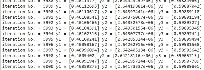
The output of the code is given below:
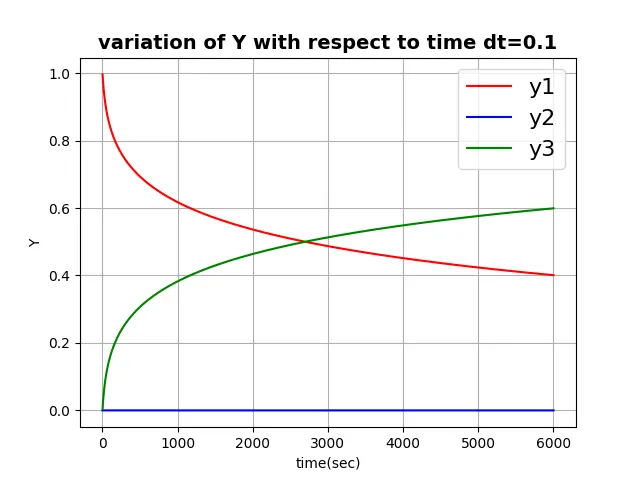
The graphical plot of solutions: