Numerical simulation of Linear Convection at different time steps using MATLAB

AIM: Study the effects of time step sizes for a 1D linear convection problem.

GOVERNING EQUATION:

The general formula for 1D convection is given by

Discretizing the above equation in terms of explicit scheme where the first term is discretized with respect to time and the second term with respect to space gives:

N represents the present time step.

U represents velocity.

BOUNDARY CONDITIONS AND INPUT PARAMETER:

1. Length of domain L=1m
2. Initial velocity profile is a step function

V=2m/s, 0.1<x<0.3

V=1m/s, everywhere

3. C=1
4. Time steps =0.01
5. U(1)=1m/s
6. Forward differencing for time derivative and backward differencing for space terms

OBJECTIVE: To observe the velocity profile at different timesteps and effect of numerical diffusion.

ALGORITHM:

1. The main program calls the function named ‘linear_convection_at_different_time_steps()’ 4 times with respect to different time steps 1e-1,1e-2,1e-3,1e-4.
2. Inside the function call statement, the variables for the linear convection terms are defined.
3. Along with the variable declaration two more function call is provided inside the main function block to compute the starting and ending node for a defined no of grid points. This resembles a nested function call.
4. After calling the values of the secondary function, the boundary conditions are defined.
5. Outer for loop marching wrt time and inner loop marching wrt grid spacing is defined.
6. With respect to changed value of time steps, the function is called repetitively along with function declared within function block.
7. The value of simulation time, final and initial velocity are stored in the main program block after the function is compiled.
8. Different velocity plots wrt different time steps are plotted.
9. The simulation time for each different time steps are compared in a bar plot.

the program code for the above algorithm is given below

MATLAB CODE:

the main program code

%%%%%%%%%%%%%%%%%linear convection problem with different time steps
%%%%%%% dt=[1e-1,1e-2,1e-3,1e-4]
%%%%%%%%This program implements two function call
%%%%%%%%%first function call in the main program
%%%%%%%%%second function call inside function named'linear_convection_at_time_step'
clc
clear all
close all
%%%%%%%%%%%%%%%%%%%%%%%%%%%%%%%%%%%%%%%%%%%%%%%%%%%%%%%%%%
%%%%%%%%%%%% function call%%%%%%%%%%
%%%%%%%%%%%for time step 1e-1
[simulation_time1, u_final_1, u_initial_1, x1]=linear_convection_at_time_step(1e-1);
%%%%%%%%%%%for time step 1e-2
[simulation_time2, u_final_2, u_initial_2, x2]=linear_convection_at_time_step(1e-2);
%%%%%%%%%%%for time step 1e-3
[simulation_time3, u_final_3, u_initial_3, x3]=linear_convection_at_time_step(1e-3);
%%%%%%%%%%%for time step 1e-4
[simulation_time4, u_final_4, u_initial_4, x4]=linear_convection_at_time_step(1e-4);
%%%%%%%%%%%%%%%%%%%%%%%%%%%%%%%%%%%%%%%%%%%%%%%%%%%%%%%%%%%%%%%%%%%%%
%%%%%%%%%%%%%%%%plotting functions%%%%%%%%%%%%%%%%%
figure(1)
%%%%%%%%%%plot for time step 1e-1
plot(x1,u_final_1,'b','linewidth',0.7)%final velocity profile
grid on
hold on 
plot(x1,u_initial_1,'color','r','linewidth',1)%initial velocity profile
axis([0 1 0 2.1])
xlabel('grid spacing')
ylabel('velocity')
legend('final velocity profile','initial velocity profile')
title('linear convection problem at timestep 1e-1')
%%%%%%%%%%%%%%%%%%%%%%%%%%%%%%%%%%%%
figure(2)
%%%%%%%%%%plot for time step 1e-2
plot(x2,u_final_2,'b','linewidth',0.7)%final velocity profile
hold on
grid on
plot(x2,u_initial_2,'color','r','linewidth',1)%initial velocity profile
xlabel('grid spacing')
ylabel('velocity')
axis([0 1 0 2.1])
legend('final velocity profile','initial velocity profile')
title('linear convection problem at timestep 1e-2')
%%%%%%%%%%%%%%%%%%%%%%%%%%%%%%%%%%%%
figure(3)
%%%%%%%%%%plot for time step 1e-3
plot(x3,u_final_3,'linewidth',0.7)%final velocity profile
hold on
grid on
plot(x3,u_initial_3,'color','r','linewidth',1)%initial velocity profile
xlabel('grid spacing')
ylabel('velocity')
axis([0 1 0 2.1])
legend('final velocity profile','initial velocity profile')
title('linear convection problem at timestep 1e-3')
%%%%%%%%%%%%%%%%%%%%%%%%%%%%%%%%%%%%
figure(4)
%%%%%%%%%%plot for time step 1e-4
plot(x4,u_final_4,'linewidth',0.7)%final velocity profile
hold on
grid on
plot(x4,u_initial_4,'color','r','linewidth',1)%initial velocity profile
xlabel('grid spacing')
ylabel('velocity')
axis([0 1 0 2.1])
legend('final velocity profile','initial velocity profile')
title('linear convection problem at timestep 1e-4')
%%%%%%%%%%%%%%%%%%%%%%%%%%%%%%%%%%%%%%%%%
%%%%%%%%%%%%%comparison between final and initial velocity profile at different time steps
figure(5)
plot(x1,u_initial_1,'color','r','linewidth',2)
hold on
grid on
plot(x1,u_final_1,'b',x1,u_final_2,'g',x1,u_final_3,'m',x1,u_final_4,'k')
grid on
xlabel('grid spacing')
ylabel('velocity')
axis([0 1 0 2.1])
legend('initial velocity','velocity at 1e-1','velocity at 1e-2','velocity at 1e-3','velocity at 1e-4')
title('comparison between final and initial velocity profile at different time steps')
%%%%%%%%%%%%%%%%%%%%%%%%%%%%%%%%%%%%%%%%%%%%%%%%%bar plot%%%%%%%%%%%%%%%%%%
%%%%%%%%%%%%Comparison between simulation time and time steps%%%%%%%%%%%%%
figure(6)
computation_time=[simulation_time1 simulation_time2 simulation_time3 simulation_time4];
c=categorical({'dt=1e-1','dt=1e-2','dt=1e-3','dt=1e-4'});
bar(c,computation_time,'facecolor',[0 0.8 0.8])
xlabel('time steps')
ylabel('simulation time')

function block

function [time, uold, u_initial,x]=linear_convection_at_time_step(dt)
%%%%%solving linear convection problem
%%%%%du/dt=-c*du/dx
%length of the domain
l=1;
c=1; 
%define the grid points
n=80;% no of grid points 
%define the mesh
x=linspace(0,l,n);
dx=x(2)-x(1);%grid spacing
%functioncall to calculate the starting node 
n_start=finding_starting_node(x,dx);
%functioncall to calculate the end node
n_end=finding_end_node(x,dx);
%define velocity at the node points
u=ones(1,n);
u(n_start:n_end)=2;
uold=u;
u_initial=u;
%bc
u(1)=1;
%no of time steps
nt=10;
tic
%%%%%%%using forward difference wrt time and backward difference wrt space
for k=1:nt%time marching steps
for i=2:n% space convergence loop
    
u(i)=uold(i)+(-c*dt/dx)*(uold(i)-uold(i-1));
end
%update velocities
uold=u;
end
time=toc;%%%computes the simulation time
end

starting node function

function output=finding_starting_node(x,dx)
output=1;
for i=1:length(x)
if x(i)<= 0.1
    output=output+1;
end 
end
end

ending node function

function output=finding_end_node(x,dx)
output=1;
for i=1:length(x)
if x(i)<= 0.3
    output=output+1;
end 
end
end

RESULTS AND DISCUSSION:

for timesteps 1e-1

The final velocity profile gets distorted at the boundary of the domain. The appearence of such instability gives rise to Gibbs phenomenon.

for timesteps 1e-2

In this time step the velocity profile is almost same as that of its initial profile. There is no drop in velocity peak profile. This is the most stable solution plot compared to other plots.

for timesteps 1e-3

the change in the velocity profile is very minimum. The boundary of the profile is seen to shift a bit in right side. The drop in peak profile is almost negligible.

for timesteps 1e-4

In this case there is no change in velocity profile, except at the corners.

velocity profiles for all combined timesteps

bar plot at different time steps

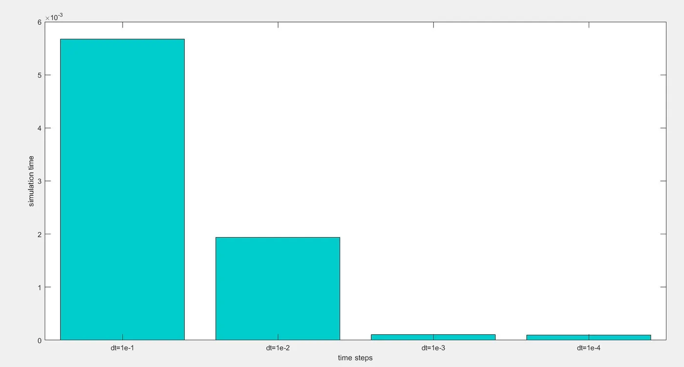
Fro this barplot it is observed that at timestep 1e-1, the simulation time is maximum because of the rise of instability. The simulation time is seen for 1e-4, where the velocity profile remains almost stagnant except at the corners.

CONCLUSION:

1. Artificial diffusion is caused due to error term in first approximation of time and space derivatives.
2. A stable velocity profile is observed at 1e-2 and inastability at 1e-1.
3. These error terms are similar to diffusion terms in navier-stokes equation.