Week 5 - Curve fitting
AIM:
To find the best fit for the given data using curve fit function.
Overview of Curve Fitting:
Curve fitting is a process of constructing a curve, or mathematical function, that has the best fit to a series of data points. It involves finding the parameters of the function that minimize the difference between the data points and the curve. This is widely used in data analysis to make predictions or understand the underlying relationships in data.
Explanation of Code:
1. Understanding popt and pcov
In the context of the curve_fit function from the scipy.optimize module:
- popt: This is an array containing the optimal values for the parameters of the fitting function that minimize the sum of the squared residuals.
- pcov: This is the estimated covariance of popt. It provides an estimate of the uncertainty of the fitted parameters.
In the context of the curve_fit function from the scipy.optimize module, pcov represents the estimated covariance of the optimal parameters (popt). Here's a breakdown of its components and how to use it: This is a 2D array where each element indicates the covariance between the -th and -th parameters. The diagonal elements provide the variance of the -th parameter estimate.
- pcov
(Parameter Covariance Matrix): This is a 2D array where each element pcov[i,
j] indicates the covariance between the i-th and j-th
parameters. The diagonal elements pcov[i, i] provide the variance
of the i-th parameter estimate.
- Variance
and Standard Deviation: The variance of a parameter estimate gives us
an idea of the spread of the parameter values. To get the standard
deviation (a measure of uncertainty) of each parameter, take the square
root of the diagonal elements of pcov.
2. np.array(temperature)
The function np.array(temperature) converts the list temperature into a NumPy array. This is useful because NumPy arrays provide more efficient operations for numerical computations compared to Python lists.
3. The * in *popt
The * operator in *popt unpacks the values in the popt array. It allows you to pass the elements of popt as separate arguments to the function linear or cubic.
4. Fitting Linear and Cubic Polynomials
The provided code fits both a linear and a cubic polynomial to the Cp data. Below is the code with explanations:
import numpy as np
import matplotlib.pyplot as plt
from scipy.optimize import curve_fit
from sklearn.metrics import r2_score
# Define the linear and cubic functions
def linear(t, a, b):
return a * t + b
def cubic(t, a, b, c, d):
return a * (t**3) + b * (t**2) + c * t + d
import numpy as np
import matplotlib.pyplot as plt
from scipy.optimize import curve_fit
from sklearn.metrics import r2_score
# Define the linear and cubic functions
def linear(t, a, b):
return a * t + b
def cubic(t, a, b, c, d):
return a * (t**3) + b * (t**2) + c * t + d
# Function to read the data file
def read_file():
temperature = []
cp = []
for line in open('data', 'r'):
values = line.split(',')
temperature.append(float(values[0]))
cp.append(float(values[1]))
return [temperature, cp]
# Read data
temperature, cp = read_file()
# Fit linear polynomial
popt_linear, pcov_linear = curve_fit(linear, temperature, cp)
fit_cp_linear = linear(np.array(temperature), *popt_linear)
# Fit cubic polynomial
popt_cubic, pcov_cubic = curve_fit(cubic, temperature, cp)
fit_cp_cubic = cubic(np.array(temperature), *popt_cubic)
# Calculate residuals
residuals_linear = np.array(cp) - fit_cp_linear
residuals_cubic = np.array(cp) - fit_cp_cubic
# Calculate RSS
rss_linear = np.sum(residuals_linear**2)
rss_cubic = np.sum(residuals_cubic**2)
# Calculate R-squared
r2_linear = r2_score(cp, fit_cp_linear)
r2_cubic = r2_score(cp, fit_cp_cubic)
# Print RSS and R-squared values
print(f"Linear Fit RSS: {rss_linear}, R²: {r2_linear}")
print(f"Cubic Fit RSS: {rss_cubic}, R²: {r2_cubic}")
# Plotting the results
plt.figure(1)
plt.plot(temperature, cp, color='b', linewidth=3)
plt.plot(temperature, fit_cp_linear, color='r', linewidth=3)
plt.title('Linear Polynomial')
plt.legend(['Actual data', 'Curve fit'])
plt.xlabel('Temperature')
plt.ylabel('Cp')
plt.figure(2)
plt.plot(temperature, cp, color='b', linewidth=3)
plt.plot(temperature, fit_cp_cubic, color='g', linewidth=3)
plt.title('Cubic Polynomial')
plt.legend(['Actual data', 'Curve fit'])
plt.xlabel('Temperature')
plt.ylabel('Cp')
plt.figure(3)
plt.plot(temperature, cp, color='b', linewidth=2)
plt.plot(temperature, fit_cp_linear, color='r', linewidth=3)
plt.plot(temperature, fit_cp_cubic, color='g', linewidth=3)
plt.title('Linear vs Cubic')
plt.legend(['Actual data', 'Linear', 'Cubic'])
plt.xlabel('Temperature')
plt.ylabel('Cp')
plt.show()
Explanation of Results
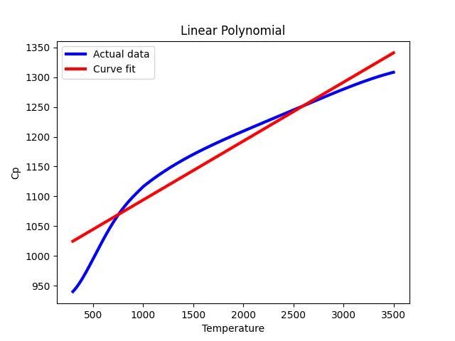
- Linear Fit: The linear fit attempts to model the relationship between temperature and Cp with a straight line. This is suitable if the data shows a linear trend.
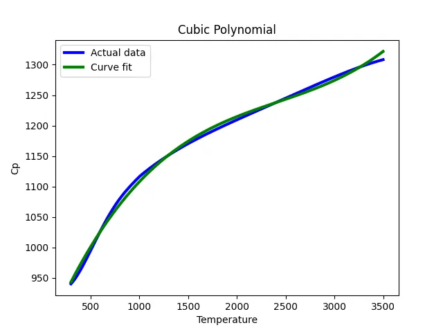
- Cubic Fit: The cubic fit uses a third-degree polynomial, which can capture more complex relationships and curvature in the data.
5. Making the Curve Fit Perfect
To improve the fit, consider the following steps:
- Higher-Order Polynomials: Use higher-degree polynomials if the cubic fit is insufficient.
- Different Models: Try different types of models (e.g., exponential, logarithmic) depending on the data pattern.
- Data Preprocessing: Clean the data, remove outliers, and normalize if necessary.
- Regularization: Apply regularization techniques to avoid overfitting when using higher-degree polynomials.
6. Empirical Evaluation
To empirically evaluate the fit, calculate the residuals and use metrics such as:

- Residual Sum of Squares (RSS): Measures the total deviation of the response values from the fit.
- R-squared (R²): Indicates the proportion of variance explained by the model.
CONCLUSION :
- Objective: Fit a linear and cubic polynomial to Cp data and evaluate the fit quality.
- Methods: Utilized scipy.optimize.curve_fit to fit the models and matplotlib.pyplot for visualization.
- Linear fit: Provides a basic approximation.
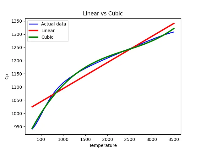
- Cubic fit: Captures more complex trends and fits the data better.
- Evaluation: Empirical metrics (RSS and R²) show the cubic fit has lower residuals and higher R², indicating a better fit.
- The cubic polynomial provides a significantly better fit compared to the linear model, suggesting it captures the underlying data trend more accurately. Further improvements can be achieved by exploring different models and refining data preprocessing steps.