PARSING NASA THERMODYNAMIC DATA

AIM :

To perform File parsing on the given data file using MATLAB.

OBJECTIVE :

• To write a function that extracts the 14 co-efficients and calculates the enthalpy, entropy and specific heats for all the species using NASA thermodynamic data.
• To calculate the molecular weight of each species .
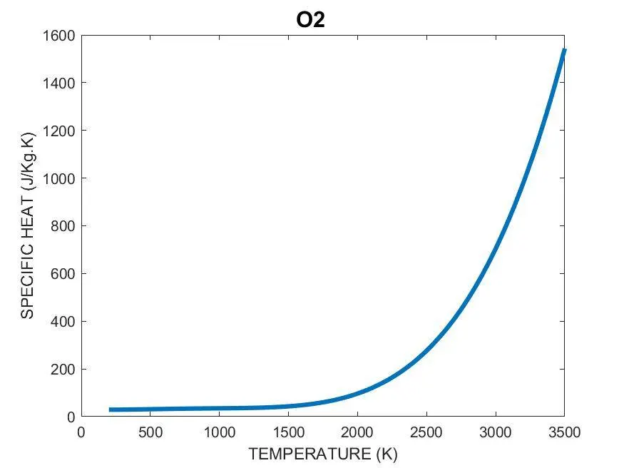
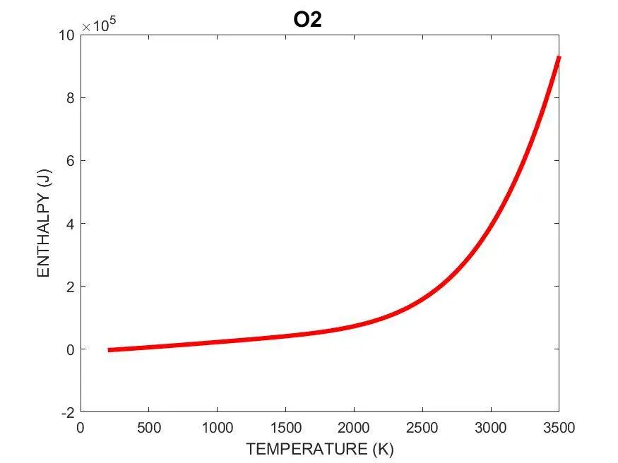
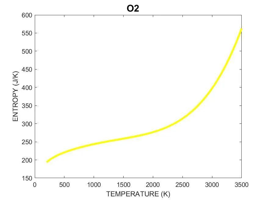
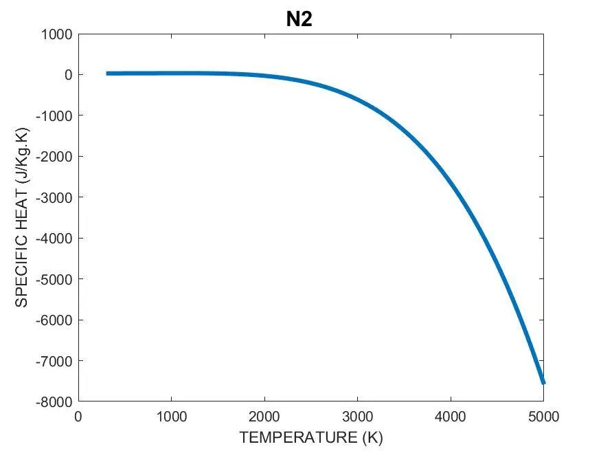
• To plot the Cp, Enthalpy and Entropy for the local temperature range specific for each species and save the plots as images with appropriate names and dump them in separate folders for each species with suitable name.

FILE PARSING :

The process of "parsing" can be described as reading in a data stream of some sort and building an in-memory model or representation of the semantic content of that data, in order to facilitate performing some kind of transformation on the data.

This process enables you to convert data from an external file into PeopleSoft data and place it into tables in your Campus Solutions database.

The external file can be a delimited file or a flat file. It can be a simple file with one row type or a complex file with several row types.

NASA came up with polynomials that can be used to evaluate thermodynamic properties such as Cp, H and S. They have also documented the co-efficients that are required to evaluate these polynomials for numerous species using the data file and executed through MATLAB.

CODE & EXPLANATION :

File parsing was performed for the given data through a code which is given below.

The code was broke down into small snippets for explanation and the entire code is also attached below.

Initially the fopen command was used to read the data file and to extract the information fgetl command was used.

f1 = fopen('THERMO.dat','r')
fgetl(f1)
tline = fgetl(f1);
A1 = strsplit(tline,' ');

Using strsplit command we can get the global temperatures , str2double command is used to convert the string into integers.

The next three lines of commentrs was incorporated using for loop.

A1 = strsplit(tline,' ');
Global_low_temp = str2double(A1{2})
Global_mid_temp = str2double(A1{3})
Global_high_temp = str2double(A1{4})

for i = 1:3
    comments = fgetl(f1);
end

Here the species name was segregated and the local temperatures that are specific to each species was extracted.

str2double command is used to convert them as integers.

species= fgetl(f1);
temp = strfind(species,'.');
 
species_name =species(1:6)

    species(52-4:52+3);
    low_temp = species(52-3:52+3);
    low_temp = str2double(low_temp)
    
    species(62-3:62+3);
    high_temp = species(62-4:62+3);
    high_temp = str2double(high_temp)
    
    species(72-4:72+3);
    med_temp = species(72-4:72+3);
    med_temp = str2double(med_temp)
   

All the 14 coefficients required for the further calculation were extracted using findstr command .

They were converted into integers using str2double command and these coefficients were saved under their respective names.

coeff_line_1= fgetl(f1);
    A1= findstr(coeff_line_1,'E');
   
    C1 = coeff_line_1(1:A1(1)+3);
    C1 = str2double(C1);
    
    C2 = coeff_line_1(A1(1)+4:A1(2)+3);
    C2 = str2double(C2);
    
    C3 = coeff_line_1(A1(2)+4:A1(3)+3);
    C3 = str2double(C3);
    
    C4 = coeff_line_1(A1(3)+4:A1(4)+3);
    C4 = str2double(C4);
    
    C5 = coeff_line_1(A1(4)+4:A1(5)+3);
    C5 = str2double(C5);
    
    
    coeff_line_2 = fgetl(f1);
    A2= findstr(coeff_line_2,'E');
    
    C6 = coeff_line_2(1:A2(1)+3);
    C6 = str2double(C6);
    
    C7 = coeff_line_2(A2(1)+4:A2(2)+3);
    C7 = str2double(C7);
    
    C8 = coeff_line_2(A2(2)+4:A2(3)+3);
    C8 = str2double(C8);
    
    C9 = coeff_line_2(A2(3)+4:A2(4)+3);
    C9 = str2double(C9);
    
    C10 = coeff_line_2(A2(4)+4:A2(5)+3);
    C10 = str2double(C10);
    
   
    coeff_line_3 = fgetl(f1);
    A3 = findstr(coeff_line_3,'E');
    
    C11 = coeff_line_3(1:A3(1)+3);
    C11 = str2double(C11);
    
    C12 = coeff_line_3(A3(1)+4:A3(2)+3);
    C12 = str2double(C12);
    
    C13 = coeff_line_3(A3(2)+4:A3(3)+3);
    C13 = str2double(C13);
    
    C14 = coeff_line_3(A3(3)+4:A3(4)+3);
    C14 = str2double(C14);

These functions were used inorder to calculate the values of Specific Heat, Enthalpy, Entropy and Molecular weight.

[Cp,H,S] = inputs(T,R,med_temp,C1,C2,C3,C4,C5,C6,C7,C8,C9,C10,C11,C12,C13,C14);

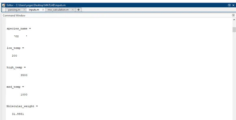
Molecular_weight = mw_calculation(species_name)

These were the verious commands used for plotting three different graphs for the given species using the extracted data.

The plot command is used to perform these operations.

The plots are represented along with labels and title.

    figure(1)
    plot(T,Cp,'linewidth',3)
    xlabel('TEMPERATURE')
    ylabel('SPECIFIC HEAT')
    title(species_name,'fontsize',15)
    
    figure(2)
    plot(T,H,'linewidth',3,'color','r')
    xlabel('TEMPERATURE')
    ylabel('ENTHALPY')
    title(species_name,'fontsize',15)
    
    figure(3)
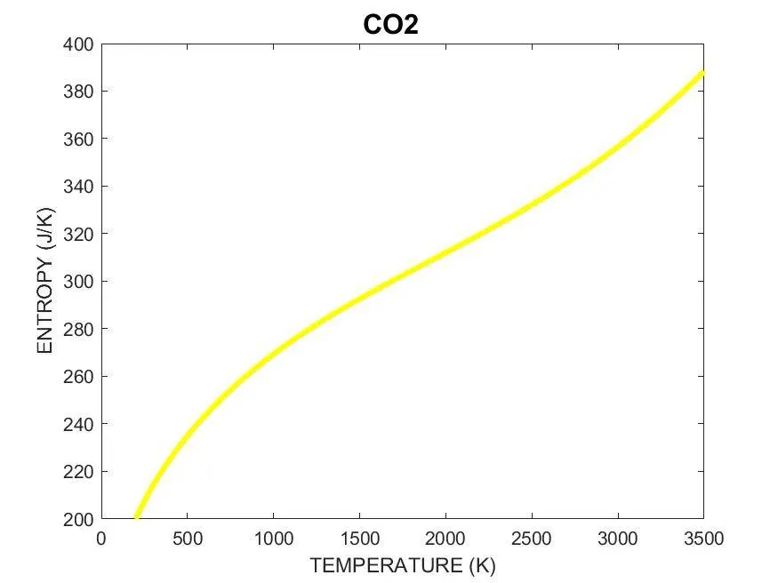
    plot(T,S,'linewidth',3,'color','y')
    xlabel('TEMPERATURE')
    ylabel('ENTROPY')
    title(species_name,'fontsize',15)

The entire code was placed under a for loop.

This loop helps us to perform the same set of operations for all the given species in the data file.

Finally all the plots were saved under specific directories for specific species which was created using mkdir command and cd command was used to change the directory inorder to save the plots in their individual folders ,of the species.

Then the directory was changed back to the original directory of the program for the seamless execution of the code.

MAIN CODE :

close all
clear all
clc

% Data file Input
f1 = fopen('THERMO.dat','r')
fgetl(f1)
tline = fgetl(f1);

% Retriving the Global temperatures
A1 = strsplit(tline,' ');
Global_low_temp = str2double(A1{2})
Global_mid_temp = str2double(A1{3})
Global_high_temp = str2double(A1{4})

% Printing the comments from the file 
for i = 1:3
    comments = fgetl(f1);
end

for i = 1:53

 % Obtaining the species information   
 species= fgetl(f1);
 temp = strfind(species,'.');
 
 species_name =species(1:6) % species name is derived

     % Calculating local temperatures  
    species(52-4:52+3);
    low_temp = species(52-3:52+3);
    low_temp = str2double(low_temp)
    
    species(62-3:62+3);
    high_temp = species(62-4:62+3);
    high_temp = str2double(high_temp)
    
    species(72-4:72+3);
    med_temp = species(72-4:72+3);
    med_temp = str2double(med_temp)
   
    % Extracting the coefficients
    coeff_line_1= fgetl(f1);
    A1= findstr(coeff_line_1,'E');
   
    C1 = coeff_line_1(1:A1(1)+3);
    C1 = str2double(C1);
    
    C2 = coeff_line_1(A1(1)+4:A1(2)+3);
    C2 = str2double(C2);
    
    C3 = coeff_line_1(A1(2)+4:A1(3)+3);
    C3 = str2double(C3);
    
    C4 = coeff_line_1(A1(3)+4:A1(4)+3);
    C4 = str2double(C4);
    
    C5 = coeff_line_1(A1(4)+4:A1(5)+3);
    C5 = str2double(C5);
    
    
    coeff_line_2 = fgetl(f1);
    A2= findstr(coeff_line_2,'E');
    
    C6 = coeff_line_2(1:A2(1)+3);
    C6 = str2double(C6);
    
    C7 = coeff_line_2(A2(1)+4:A2(2)+3);
    C7 = str2double(C7);
    
    C8 = coeff_line_2(A2(2)+4:A2(3)+3);
    C8 = str2double(C8);
    
    C9 = coeff_line_2(A2(3)+4:A2(4)+3);
    C9 = str2double(C9);
    
    C10 = coeff_line_2(A2(4)+4:A2(5)+3);
    C10 = str2double(C10);
    
   
    coeff_line_3 = fgetl(f1);
    A3 = findstr(coeff_line_3,'E');
    
    C11 = coeff_line_3(1:A3(1)+3);
    C11 = str2double(C11);
    
    C12 = coeff_line_3(A3(1)+4:A3(2)+3);
    C12 = str2double(C12);
    
    C13 = coeff_line_3(A3(2)+4:A3(3)+3);
    C13 = str2double(C13);
    
    C14 = coeff_line_3(A3(3)+4:A3(4)+3);
    C14 = str2double(C14);
    
    % Calculating the optimum temperature
    T  = linspace(low_temp,high_temp,100);
    R  = 8.314 ; % Universal gas constant
    
    % Function calling to obtain Cp,H,S values
    [Cp,H,S] = inputs(T,R,med_temp,C1,C2,C3,C4,C5,C6,C7,C8,C9,C10,C11,C12,C13,C14);
    
    % Plotting the various curves 
    figure(1)
    plot(T,Cp,'linewidth',3)
    xlabel('TEMPERATURE (K)')
    ylabel('SPECIFIC HEAT (J/Kg.K)')
    title(species_name,'fontsize',15)
    
    figure(2)
    plot(T,H,'linewidth',3,'color','r')
    xlabel('TEMPERATURE (K)')
    ylabel('ENTHALPY (J)')
    title(species_name,'fontsize',15)
    
    figure(3)
    plot(T,S,'linewidth',3,'color','y')
    xlabel('TEMPERATURE (K)')
    ylabel('ENTROPY (J/K)')
    title(species_name,'fontsize',15)
    
    %Creating a folder to save the plots 
    mkdir('C:UsersyogesDesktopMATLABNASA File parising',species_name)
    folder = (['C:UsersyogesDesktopMATLABNASA File parising',species_name]);
    cd(folder)
    
    % Saving the plots as images
    saveas(1,'Temperature vs Specific Heat.jpg')
    saveas(2,'Temperature vs Enthalpy.jpg')
    saveas(3,'Temperature vs Entropy.jpg')
    
    % Changing of directory 
    cd('C:UsersyogesDesktopMATLAB')
    
    % Function calling to obtain molecular weight 
    Molecular_weight = mw_calculation(species_name)
    
end
    
fclose(f1)

FUNCTIONS :

In this program there were 2 functions used. These functions helped in the simpification of the main program.

FUNCTION 1 : Calculation of Cp,H & S

The specific heat , enthalpy and the entropy were calculated using the formula,

where Cp - Specific Heat (J/Kg.K)

H - Enthalpy (J)

S - Entropy (J/K)

R - Universal Gas constant

T - Optimum temperature

and a1-a7 were the coefficients.

Here in this program the coefficients were represented as C1 to C14 where, the first 7 coefficients have used local high temperature and the remaining 7 coefficiets have used local low temperature for processing.

By using this function the values were calculated on receiving the inputs from the main program and the output was passed on to the main program when the function is called.

The file is saved by using the same name as the function.

% Calculating Specific heat, Enthalpy & Entropy
function [Cp,H,S] = inputs(T,R,med_temp,C1,C2,C3,C4,C5,C6,C7,C8,C9,C10,C11,C12,C13,C14)

for i = 1:length(T)
    if T(i)>T
        % High temperature coefficients 
        Cp = (C1 + C2.*T + C3.*T.^2 + C4.*T.^3 + C5.*T.^4)*R;
        H  = (C1 + (C2.*T)./2 + (C3.*T.^2)./3 + (C4.*T.^3)./4 + (C5.*T.^4)./5 + C6./T).*T.*R;
        S  = (C1.*log(T) + C2.*T + (C3.*T.^2)./2 + (C4.*T.^3)./3 + (C5.*T.^4)./4 + C7 )*R ;
        
    else
        
        % Low temperature coefficients
        Cp = (C8 + C9.*T + C10.*T.^2 + C11.*T.^3 + C12.*T.^4)*R;
        H  = (C8 + (C9.*T)./2 + (C10.*T.^2)./3 + (C11.*T.^3)./4 + (C12.*T.^4)./5 + C13./T).*T.*R;
        S  = (C8.*log(T) + C9.*T + (C10.*T.^2)./2 + (C11.*T.^3)./3 + (C12.*T.^4)./4 + C14 )*R ;
        
    end
end
end

FUNCTION 2 : Calculation of Molecular weight

The Molecular weight of a substance can be calculated using the following steps

• Determine the molecular formula of the molecule.
• Use the periodic table to determine the atomic weighty of each element in the molecule.
• Multiply each element's atomic mass by the number of atoms of that element in the molecule.
• Add these values together for each different atom in the molecule.

The atomic weights of the associated elements belonging to the species were given as inputs.

Then the for loop was used to calculate the molecular weigfht of each species individually.

further the strcmp command was used under the if statement to compare the species with the elements that were given as inputs and their moelcular weight is calculated and converted into integers using str2double command.

% Molecular weight calculation
function Molecular_weight = mw_calculation(species_name)

species = (species_name);

% Defining the respective atomic weights
elements = ['H','C','O','N','A','S'];
atomic_weight = [1.00784,12.0096,15.99903,14.00643,39.948,32.059];

Molecular_weight = 0;

for i = 1:length(species)
    for j = 1:length(elements)
        if strcmp(species(i),elements(j))
            Molecular_weight = Molecular_weight + atomic_weight(j);
            a = j;
            
        end
    end
    
    n = str2double(species(i));
    if n>1;
        Molecular_weight = Molecular_weight + atomic_weight(a)*(n-1);
    end
end
end

OUTPUTS :

• Screenshot of the window where all the folders are saved.

• PLOTS FOR O2

• PLOTS FOR N2

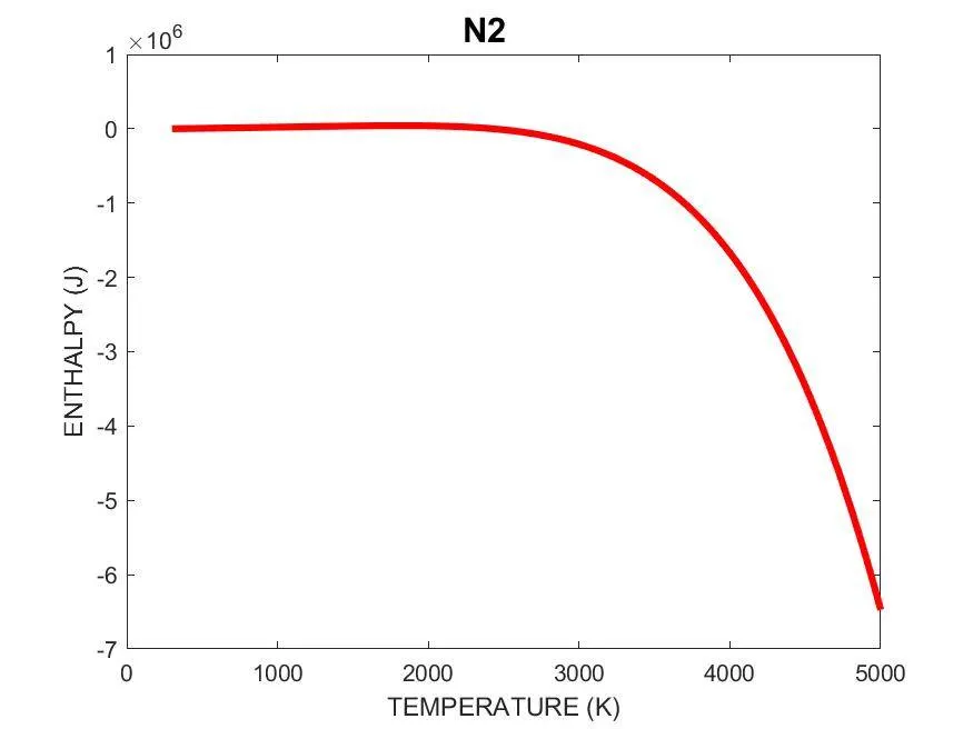
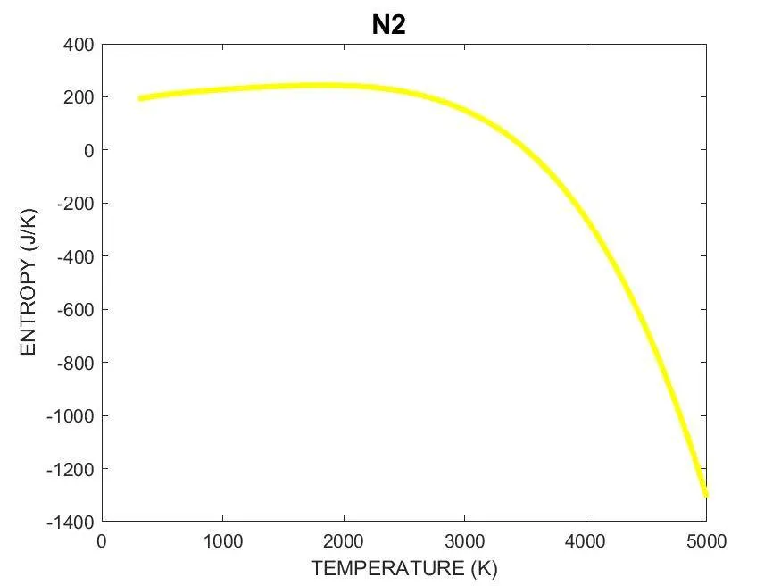
• PLOTS FOR CO2

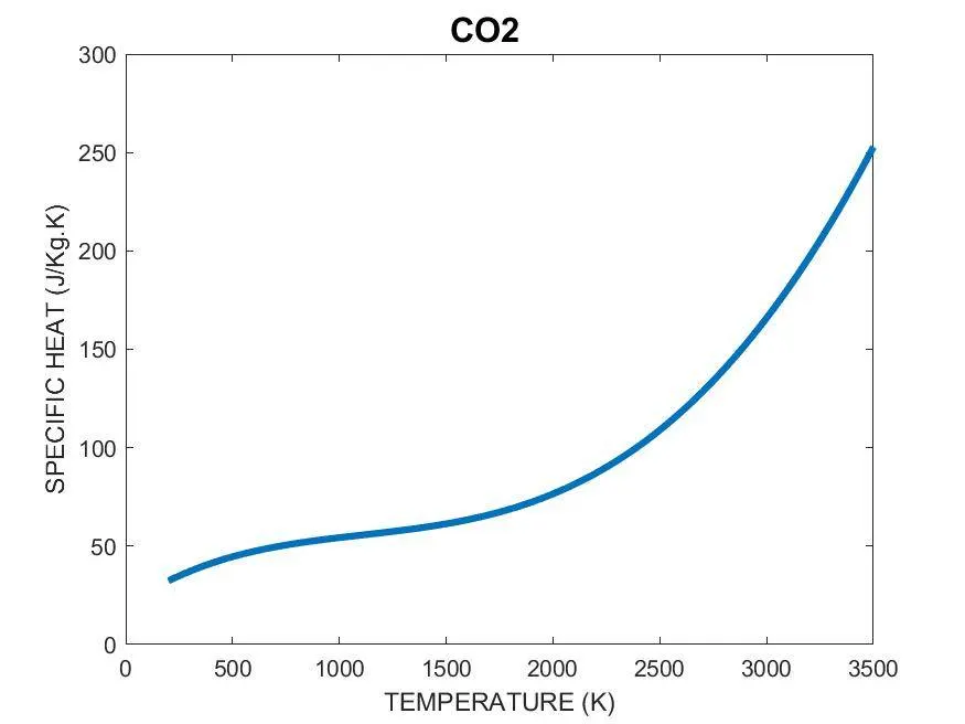
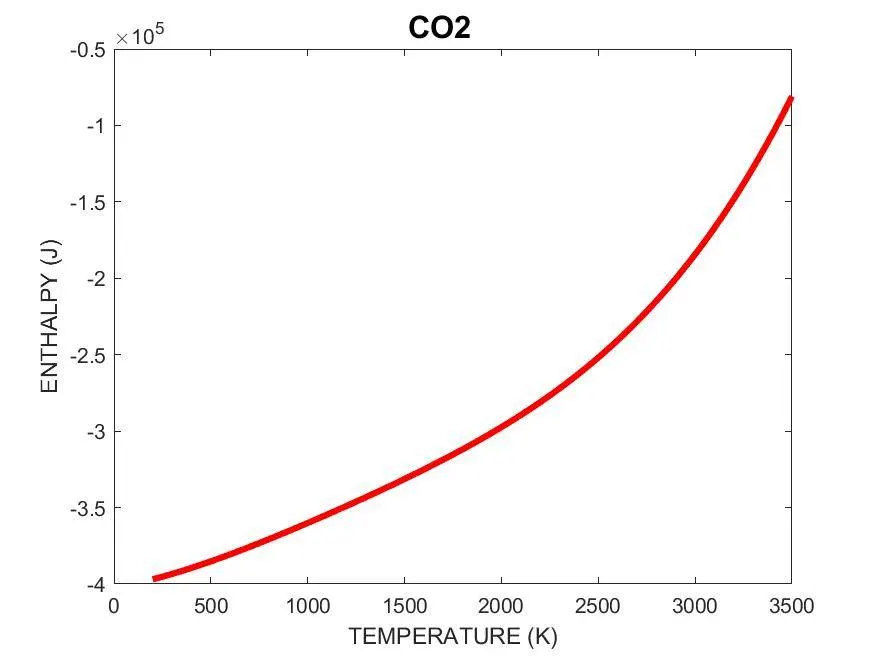
• MOLECULAR WEIGHT CALCULATION :

CONCLUSION :

The File Parsing process was performed just by taking the input from the given data file.

It returns the values of specific heat, enthalpy and entropy as outputs.

File Parsing holds lots of benefits that includes

• Eradication of repetitive data entry.
• Removal of data processing errors.
• Increase in employee productivity.
• Automatic fulfilment of company or industry compliance procedures.

Thus file parsing is an effective mesaure which can be formulated using MATLAB.

REFERENCES :

• https://www.mathworks.com/help/matlab/ref/mkdir.html?searchHighlight=mkdir&s_tid=doc_srchtitle
• https://www.mathworks.com/help/matlab/ref/cd.html