GENETIC ALGORITHM - MATLAB
AIM :
To optimise the stalagmite function and find the global maxima of the function using MATLAB.
OBJECTIVE :
To Explain the concept of GA in MATLAb.
To plot graphs for all 3 studies.
To plot graphs for F maximum vs Number of iterations.
ABOUT :
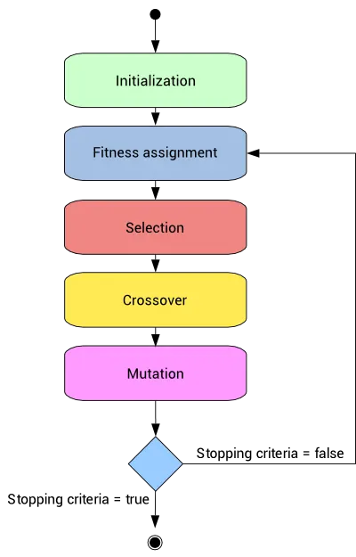
A genetic algorithm is a search heuristic that is inspired by Charles Darwin's theory of natural evolution. This algorithm reflects the process of natural selection where the fittest individuals are selected for reproduction in order to produce offspring of the next generation.
Five phases are considered in a genetic algorithm.
- Initial population
- Fitness function
- Selection
- Crossover
- Mutation
INITIAL POPULATION :
The process begins with a set of individuals which is called a Population. Each individual is a solution to the problem you want to solve.
An individual is characterized by a set of parameters known as Genes.
FITNESS FUNCTION :
The fitness function determines how fit an individual is , it gives a fitness score to each individual. The probability that an individual will be selected for reproduction is based on its fitness score.
In short it is the ability of an individual to compete with other individuals.
SELECTION :
The idea of selection phase is to select the fittest individuals and let them pass their genes to the next generation.
Two pairs of individuals are selected based on their fitness scores. Individuals with high fitness have more chance to be selected for reproduction.
The selection function chooses parents for the next generation based on their scaled values from the fitness scaling function. The scaled fitness values are called the expectation values.
An individual can be selected more than once as a parent, in which case it contributes its genes to more than one child
REPRODUCTION :
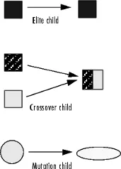
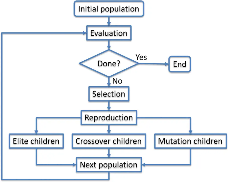
Reproduction options control how the genetic algorithm creates the next generation. The two ways of reproduction include,
Cross Over :
Crossover is the most significant phase in a genetic algorithm. For each pair of parents to be mated, a crossover point is chosen at random from within the genes.
Types of crossover include
- One - Point Crossover
- Two - Point Crossover
- Order Crossover (OX)
- Partially Mapped Crossover (PMX)
- Cycle Crossover (CX)
Mutation :
In certain new offspring formed, some of their genes can be subjected to a mutation with a low random probability. This implies that some of the bits in the bit string can be flipped.
These children are formed by applying random changes to a single individual in the current generation to create a child.
FLOWCHART REPRESENTING GA :
CODE & EXPLANATION :
Initially two vectors were defined using the linspace command. A 2D mesh wa created from the two vectors to act as a medium to find the maxima of the function.
The meshgrid command was used to create the required 2D mesh.
A for loop was created to loop for 50 instances and at each instance ,the value of fitness function was calculated.
The Fitness function consists of certain equations whichwas defined in the function 'stalagmite.m', which was called inside the for loop.
Further the surface was created using the surfc command which provides the contour of the generated surface,the shading interp function was used to smoothen the generated plot.
A subplot command was used to have tow plots in the same space.
The tic-toc command was used to calculate the study time.
A negative sign was used inside the surfc command for thge function f inorder to obtain a surface upside down.
CODE :
close all
clear all
clc
 x=linspace(0,0.6,150);
 y=linspace(0,0.6,150);
 cases = 50; % Number of iterations to be performed

 % Creating a 2D mesh
 [xx,yy]=meshgrid(x,y);

 % Creating the plot for the function
 for i = 1 : length(xx)
     for j = 1: length(yy)

         input_vector(1) = xx(i,j);
         input_vector(2) = yy(i,j);
         f(i,j) = stalagmite(input_vector); % function calling
     end
 end


 % Unbounded statistical behaviour

 tic % calculation of study time
 for i = 1:cases
     [input1,fopt1(i)] = ga(@stalagmite,2)
     xopt(i) = input1(1);
     yopt(i) = input1(2);
 end

 study_time1 = toc
 figure(1)
 subplot(2,1,1)
 hold on
 surfc(xx,yy,-f) % Generating the surface
 xlabel('X-axis')
 ylabel('Y-axis')
 zlabel('Function Value')
 shading interp % To smoothen the plot

 plot3(xopt,yopt,-fopt1,'marker','o','markersize',5,'markerfacecolor','r')
 title('UNBOUNDED STATISTICAL BEHAVIOUR')
 subplot(2,1,2)
 plot(-fopt1)
 xlabel('Number of Iterations')
 ylabel('Function Maximum')

 % Statistical behaviour with upper and lower bounds
 tic % calculation of study time
 for i = 1:cases
     [input2,fopt2(i)] = ga(@stalagmite,2,[],[],[],[],[0;0],[1;1]); % providing bounds
     xopt(i) = input2(1);
     yopt(i) = input2(2);
 end

 study_time2 = toc;
 figure(2)
 subplot(2,1,1)
 hold on
 surfc(xx,yy,-f) % Generating the surface
 xlabel('X-axis')
 ylabel('Y-axis')
 zlabel('Function Value')
 shading interp % smoothening the plot

 plot3(xopt,yopt,-fopt2,'marker','o','markersize',5,'markerfacecolor','r')
 title('BOUNDED STATISTICAL BEHAVIOUR')
 subplot(2,1,2)
 plot(-fopt2)
 xlabel('Number of Iterations')
 ylabel('Function Maximum')


 % Increasing the population size of GA
 options = optimoptions('ga'); % To increase the population size
 options = optimoptions(options,'populationsize',170);

 tic % calculation of study time
 for i = 1:cases
     [input3,fopt3(i)] = ga(@stalagmite,2,[],[],[],[],[0;0],[1;1],[],[],options); % Providing bounds and increasing the size
     xopt(i) = input3(1);
     yopt(i) = input3(2);
 end

 study_time3 = toc;
 figure(3)
 subplot(2,1,1) % Generating the surface
 hold on
 surfc(xx,yy,-f)
 xlabel('X-axis')
 ylabel('Y-axis')
 zlabel('Function Value')
 shading interp % smoothening the plot

 plot3(xopt,yopt,-fopt3,'marker','o','markersize',5,'markerfacecolor','r')
 title('BOUNDED STATISTICAL BEHAVIOUR WITH INCREASED POPULATION SIZE')
 subplot(2,1,2)
 plot(-fopt3)
 xlabel('Number of Iterations')
 ylabel('Function Maximum')

 Total_study_time = study_time1 + study_time2 + study_time3 ; % Study time calculation

 % Results screem

 fprintf('n RESULTS :')

 fprintf('nn STUDY 1 : UNBOUNDED STATISTICAL BEHAVIOUR ')
 fprintf(' nn STUDY TIME  ; %f',study_time1)
 fprintf('n LOCATION OF GLOBAL MAXIMA IN COORDINATES X & Y : %f ,%f',input1(1),input1(2))
 fprintf('n GLOBAL MAXIMA : %f',-(mean(fopt1)))

 fprintf('nn STUDY 2 : BOUNDED STATISTICAL BEHAVIOUR ')
 fprintf(' nn STUDY TIME  ; %f',study_time2)
 fprintf('n LOCATION OF GLOBAL MAXIMA IN COORDINATES X & Y : %f ,%f',input2(1),input2(2))
 fprintf('n GLOBAL MAXIMA : %f',-(mean(fopt2)))

 fprintf('nn STUDY 3 : BOUNDED STATISTICAL BEHAVIOUR WITH INCREASED POPULATION SIZE ')
 fprintf(' nn STUDY TIME  ; %f',study_time3)
 fprintf('n LOCATION OF GLOBAL MAXIMA IN COORDINATES X & Y : %f ,%f',input3(1),input3(2))
 fprintf('n GLOBAL MAXIMA : %f',-(mean(fopt3)))

 fprintf('n n TOTAL TIME TAKEN : %f',Total_study_time)
There are three different criteria for optimising the function
- Unbounded Statistical Behaviour
- Bounded Statistical Behaviour
- Bounded Statistical Behaviour with increased population size
Unbounded statistical behaviour :
In this case the optimum value of the fitness function was evaluated without any boundary conditions.
 % Unbounded statistical behaviour
 tic
 for i = 1:cases;
     [input1,fopt1(i)] = ga(@stalagmite,2)
     xopt(i) = input1(1);
     yopt(i) = input1(2);
 end

 study_time1 = toc
 figure(1)
 subplot(2,1,1)
 hold on
 surfc(xx,yy,-f)
 xlabel('X-axis')
 ylabel('Y-axis')
 zlabel('Function Value')
 shading interp

 plot3(xopt,yopt,-fopt1,'marker','o','markersize',5,'markerfacecolor','r')
 title('UNBOUNDED STATISTICAL BEHAVIOUR')
 subplot(2,1,2)
 plot(-fopt1)
 xlabel('Number of Iterations')
 ylabel('Function Maximum')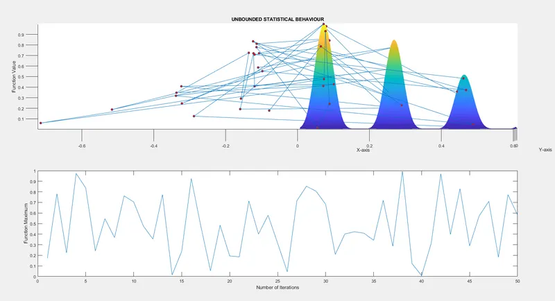
Bounded statistical behaviour :
In this case the optimum valuye of the fitness function was calculated under a specified boundary condtion.
This enables in achieving a more particular outcome of values.
 % Statistical behaviour with upper and lower bounds

 tic % calculation of study time
 for i = 1:cases
     [input2,fopt2(i)] = ga(@stalagmite,2,[],[],[],[],[0;0],[1;1]); % providing bounds
     xopt(i) = input2(1);
     yopt(i) = input2(2);
 end

 study_time2 = toc;
 figure(2)
 subplot(2,1,1)
 hold on
 surfc(xx,yy,-f) % Generating the surface
 xlabel('X-axis')
 ylabel('Y-axis')
 zlabel('Function Value')
 shading interp % smoothening the plot

 plot3(xopt,yopt,-fopt2,'marker','o','markersize',5,'markerfacecolor','r')
 title('BOUNDED STATISTICAL BEHAVIOUR')
 subplot(2,1,2)
 plot(-fopt2)
 xlabel('Number of Iterations')
 ylabel('Function Maximum')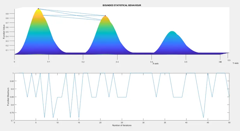
Bounded statistical behaviour with increased population size :
In this case the upper and lower bounds of the function are specified.
In addition to that the optimoptions command was used inorder to increase the population size (170).
This method provides us with the most precise outcome of the three methods.
% Increasing the population size of GA
 options = optimoptions('ga'); % To increase the population size
 options = optimoptions(options,'populationsize',170);

 tic % calculation of study time
 for i = 1:cases
     [input3,fopt3(i)] = ga(@stalagmite,2,[],[],[],[],[0;0],[1;1],[],[],options); % Providing bounds and increasing the size
     xopt(i) = input3(1);
     yopt(i) = input3(2);
 end

 study_time3 = toc;
 figure(3)
 subplot(2,1,1) % Generating the surface
 hold on
 surfc(xx,yy,-f)
 xlabel('X-axis')
 ylabel('Y-axis')
 zlabel('Function Value')
 shading interp % smoothening the plot

 plot3(xopt,yopt,-fopt3,'marker','o','markersize',5,'markerfacecolor','r')
 title('BOUNDED STATISTICAL BEHAVIOUR WITH INCREASED POPULATION SIZE')
 subplot(2,1,2)
 plot(-fopt3)
 xlabel('Number of Iterations')
 ylabel('Function Maximum')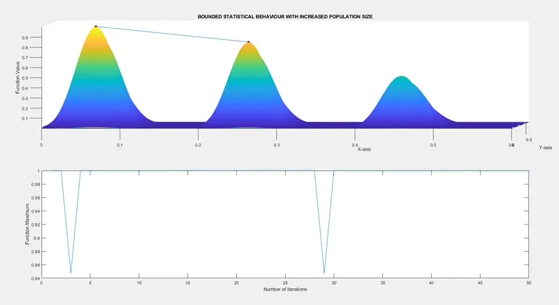
FUNCTION CODE :
This function 'stalagmite.m' consist of the fitness function.
The equations contributing to the fitness functions are,
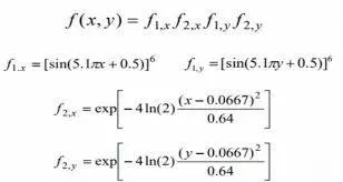
These equations were used to plot the graph in the main function.
The inputs are provided from thge meshgrid.
The negative sign was used to maximize the function.
function [f] = stalagmite(input_vector)

x = input_vector(1);
y = input_vector(2);

f1_x = (sin(5.1*pi*x  + 0.5)).^6;
f1_y = (sin(5.1*pi*y  + 0.5)).^6;


f2_x = exp(-4.*log(2)*(((x-0.0667)^2)/(0.64)));


f2_y = exp(-4.*log(2)*(((y-0.0667)^2)/(0.64)));

f = -(f1_x.*f2_x.*f1_y.*f2_y);

end
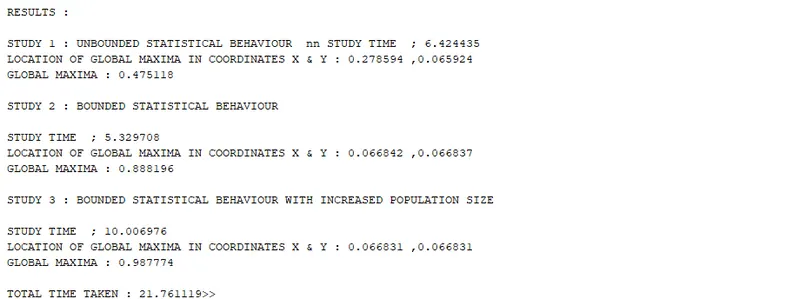
RESULTS :
The results for the optimization function are provided below
CONCLUSION :
The Graphs clearly incdicate the improvement in the optimization of the function, the bounded statistical behaaviour with increased population size gives us the most desired value.
The total study time was calculated and printed. The Global maxima of the given function has been found.
Genetic Algorithm is very useful in optimizing a given function.
GA is used in various fields such as
- Neural networks.
- Machine learning.
- Economics.
- DNA Analysis.
- Image Processing.
REFERENCE :
https://www.mathworks.com/help/gads/how-the-genetic-algorithm-works.html