RANKINE CYCLE SIMULATOR

AIM :

To create a Rankine Cycle Simulator using MATLAB.

OBJECTIVE :

To calculate the state points of the Rankine Cycle based on user inputs.

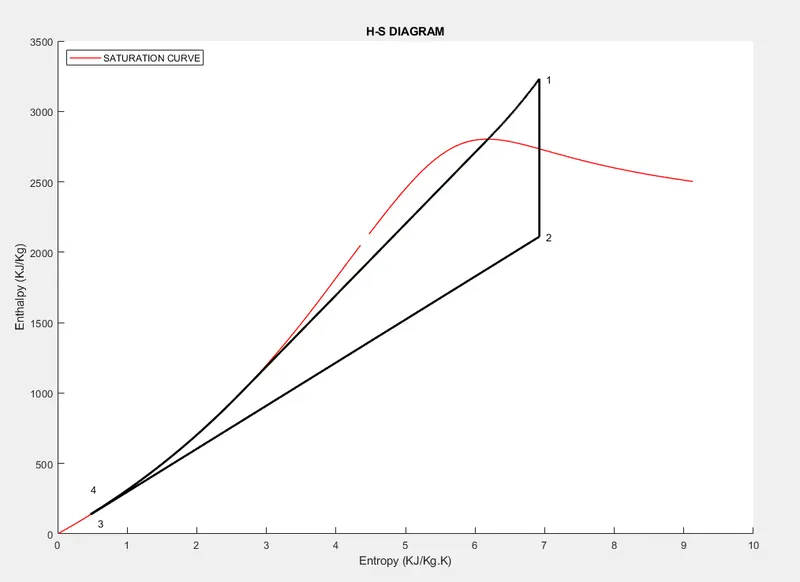
To plot the corresponding T-S and H-S plots for the given set of inputs.

To calculate

• Efficiency of the cycle.
• Net work output.
• Back work ratio.

RANKINE CYCLE :

The Rankine cycle is the fundamental operating cycle of all power plants where an operating fluid is continuously evaporated and condensed.

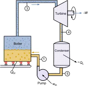
It is an ideal cycle if water passes through the four components without irreversibilities and pressure drops. The ideal Rankine cycle consists of the following four processes,

• 1-2: Constant pressure heat addition in a boiler
• 2-3: Isentropic expansion in a turbine
• 3-4: Constant pressure heat rejection in a condenser
• 4-1: Isentropic compression in a pump

Components :

Rankine cycle consists of four components namely

• Turbine
• Condenser
• Pump
• Boiler

Working :

High pressure liquid enters the boiler from the feed pump and is heated to the saturation temperature . Further addition of energy causes evaporation of the liquid until it is fully converted to saturated steam.

The vapor is expanded in the turbine, thus producing work which may be converted to electricity. In practice, the expansion is limited by the temperature of the cooling medium and by the erosion of the turbine blades by liquid entrainment in the vapor stream as the process moves further into the two-phase region. Exit vapor qualities should be greater than 90%.

The vapor-liquid mixture leaving the turbine is condensed at low pressure, usually in a surface condenser using cooling water.

In well designed and maintained condensers, the pressure of the vapor is well below atmospheric pressure, approaching the saturation pressure of the operating fluid at the cooling water temperature.

The pressure of the condensate is raised in the feed pump. Because of the low specific volume of liquids, the pump work is relatively small and often neglected in thermodynamic calculations.

Rankine cycle in power plant :

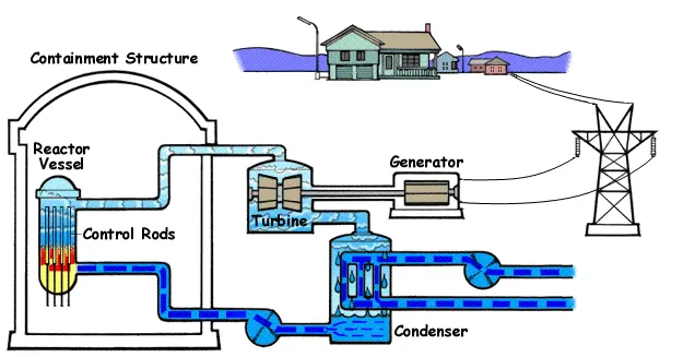
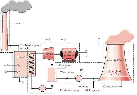
In a real power-plant cycle (the name "Rankine" cycle is used only for the ideal cycle), the compression by the pump and the expansion in the turbine are not isentropic. In other words, these processes are non-reversible, and entropy is increased during the two processes. This somewhat increases the power required by the pump and decreases the power generated by the turbine.

In particular, the efficiency of the steam turbine will be limited by water-droplet formation which leads to the decrease in the efficiency of the cycle.

As the water condenses, water droplets hit the turbine blades at high speed, causing pitting and erosion, gradually decreasing the life of turbine blades and efficiency of the turbine. The easiest way to overcome this problem is by superheating the steam.

Modifications in Rankine cycle :

In order to increase the efficiency of the cycle,certain modifications are performed.They are as follow,

• Intercooling
• Reheating
• Regeneration

CODE & EXPLANATION :

Rankine cycle is simulated using the following code given below.

The code was broke down into small snippets for explanation and the entire code is also attached below.

Initially the input data was made to receive from the user using the input command. The inlet pressure, temperature at the turbine and the inlet pressure at the condenser was obtained.

p1 = input('n nPressure at the Turbine inlet,p1(bar)=');
t1 = input('n Temperature at Turbine inlet,t1(celsius)=');
p2 = input('n Pressure at the Condenser inlet,p2(bar)=');

The inputs at the state point 1 were extracted from the 'XSteam.m' file using the following snippet.

The Enthalpy and Entropy values corresponding to the given inputs are obtained.

h1 = XSteam('h_pT',p1,t1);
s1 = XSteam('s_pT',p1,t1);

At state point 2 the entropy remains the same as like the state one since the process is isentropic.

The values of specific entropy corresponding to the fluid (sf) and the vapour (sg) states were extracted from the given data file.

Using these specific entropy values, the dryness fraction (X) of the mixture was calculated.

Further the values of specific ennthapy corresponding to the fluid (hg) and the vapour (hg) states were also extracted and using these values and the dryness fraction, the enthalpy at state point 2 was calculated.

s2 = s1;
sf2 = XSteam('sL_p',p2);
sg2 = XSteam('sV_p',p2);
x = (s2 - sf2)/(sg2-sf2);
hf2 = XSteam('hL_p',p2);
hg2 = XSteam('hV_p',p2);
h2 = hf2 + x*(hg2-hf2);

At state point 3 the pressure remains constant as point 2.

The values of enthalpy(h3) and entropy(s3) were extracted from the data file. Here the point lies on the saturation curve (liquid phase).

p3 = p2;
s3 = XSteam('sL_p',p3);
h3 = XSteam('hL_p',p3);

At state point 4 the pressure remains constant as point 1.

The entropy value here is same as the previous point as this process is isentropic.

p4 = p1 ;
s4 = s3;

Work done by the turbine was calculated using the enthalpies at inlet and exit.

The value of enthalpy at this point was calculated using the pump work.

Pump work is the product of specific volume and pressure difference.

Using this value the enthalpy at point 4 was calculated .

Here the work is done by the turbine (+ve work ) and the work inout is supplied to the pump (-ve work).

W_turbine = h1-h2;

v3 =  XSteam('vL_p',p3);
W_pump = v3*(p4-p3)*100;
h4 = W_pump + h3 ; 

Using the above obtained values , the Net work done, Heat supplied ,Heat rejected and the Efficiency of the cycle can be calculated.

Net Work done = Turbine work - Pump work

Heat supplied = h1 - h4

Heat rejected = h2 - h3

Efficiency of the Cycle = Net work / Heat supplied

Net_Work = W_turbine - W_pump;
Heat_supplied  = h1 - h4;
Hear_rejected = h2 - h3;
Eff = (Net_Work / Heat_supplied )*100;

The Back work ratio and thw Specific steam consumption of the cycle were also calculated.

BWR = W_pump/W_turbine;

SSC = 3600/(Net_Work);

The temperature at various state points were calculated.

t3 = XSteam('Tsat_p',p3);
t2 = t3;
cp4 = XSteam('Cp_ps',p4,s4);
cv4 = XSteam('Cv_ps',p4,s4);
k = cp4/cv4;
t4 = t3/((p3/p4)^((k-1)/k));

The values of Temperature , Enthaply and Entropy were calculated as the condensed fluid leaves the pump to the boiler.

t6 = XSteam('Tsat_p',p1);
t5 = t6;
s5 = XSteam('sL_p',p1);
s6 = XSteam('sV_p',p1);
h5 = XSteam('hL_p',p1);
h6 = XSteam('hV_p',p1);

For plotting the saturation curve, first the temperature values were calculated using the linspace command.

Further a for loop was used inorder to calculate the values of specific enthalpy and entropy at the fluid and vapour states respectively for each insatance of the temperature.

T = linspace(1,375,1000);

for i = 1:length(T)
sf(i) = XSteam('sL_T',T(i));
sg(i) = XSteam('sV_T',T(i));
hf(i) = XSteam('hL_T',T(i));
hg(i) = XSteam('hV_T',T(i));
end

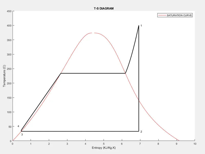
Finally the T-S diagram was plotted using the obtained values through plot command.

The Saturation curve was also plotteda and the values for the saturation curve were obtained from the given data file.

The appropriate texts to identifiy the points were done using the text command.

figure(1)
hold on
plot(sf,T,'color','r')
plot(sg,T,'color','r')
plot([s1,s2],[t1,t2],'color','black','linewidth',2)
plot([s2,s3],[t2,t3],'color','black','linewidth',2)
plot([s3,s4],[t3,t4],'color','black','linewidth',2)
plot([s4,s5],[t4,t5],'color','black','linewidth',2)
plot([s5,s6],[t5,t6],'color','black','linewidth',2)
text(s1+0.1,t1,'1')
text(s2+0.1,t2,'2')
text(s3,t3-10,'3')
text(s4-0.2,t4+15,'4')

The curved portion of the plot belonging at the super saturated region , leading to the turbine inlet was also calculated using a for loop.

The required temperature values were obtained from the given data file.

The appropriate x & y labels were also given to the plot.

The legend command was used inorder to represent the saturation curve.

sc = linspace(s6,s1,1000);

for j  = 1 : length(sc)
    Tc(j) = XSteam('T_ps',p1,sc(j));
end
plot(sc,Tc,'color','black','linewidth',2)
title('T-S DIAGRAM')
xlabel('Entropy (KJ/Kg.K)')
ylabel('Temperature (C)')
legend('SATURATION CURVE')

Then the H-s diagram was plotted using the plot command using the various obtained points along with the saturation curve.

The required titile, labels and texts were added to the plot.

figure(2)
hold on
plot(sf,hf,'color','r','linewidth',1)
plot(sg,hg,'color','r','linewidth',1)
plot([s1,s2],[h1,h2],'color','black','linewidth',2)
plot([s2,s3],[h2,h3],'color','black','linewidth',2)
plot([s3,s4],[h3,h4],'color','black','linewidth',2)
 text(s1+0.1,h1,'1')
 text(s2+0.1,h2,'2')
 text(s3+0.1,h3-60,'3')
 text(s4,h4+180,'4')
 title('H-S DIAGRAM')
 xlabel('Entropy (KJ/Kg.K)')
 ylabel('Enthalpy (KJ/Kg)')
 

Finally the curved regions of the plot were obtained using a for loop.

The necessary entropy values corresponding to the enthalpies were obtained from the given data file.

The legend ffor the saturation curve was added.

hc = linspace(h4,h5,100);
for k =1:length(hc)
    sch(k) = XSteam('s_ph',p1,hc(k));
end
plot(sch,hc,'color','black','linewidth',2)
plot([s5,s6],[h5,h6],'color','black','linewidth',2)
for l = 1:length(sc)
    hc1(l) = XSteam('h_ps',p1,sc(l));
end
 plot(sc,hc1,'color','black','linewidth',2)
 legend('SATURATION CURVE','location','northwest')

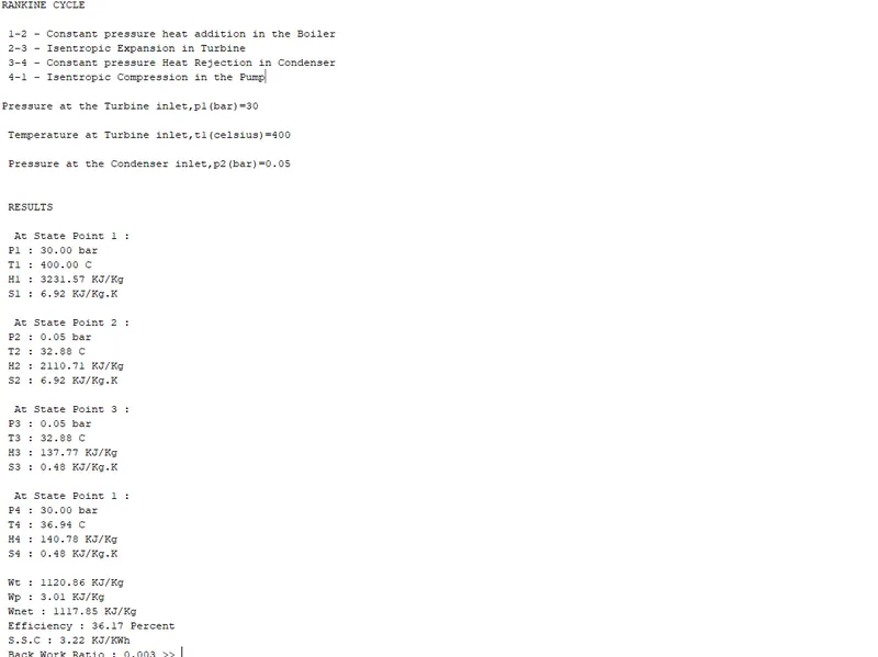
The fprintf command was used to print the processess involved in the cycle and to print all the results obtained from the simulator in a detailed manner.

This code is directly mentioned in the main program itself.

MAIN CODE :

close all
clear all
clc

fprintf('RANKINE CYCLE')

fprintf('n n 1-2 - Constant pressure heat addition in the Boiler')
fprintf('n 2-3 - Isentropic Expansion in Turbine')
fprintf('n 3-4 - Constant pressure Heat Rejection in Condenser')
fprintf('n 4-1 - Isentropic Compression in the Pump')

% User defined inputs 
p1 = input('n nPressure at the Turbine inlet,p1(bar)=');
t1 = input('n Temperature at Turbine inlet,t1(celsius)=');
p2 = input('n Pressure at the Condenser inlet,p2(bar)=');


% State 1
h1 = XSteam('h_pT',p1,t1);
s1 = XSteam('s_pT',p1,t1);

%State 2
s2 = s1; % Isentropic process
sf2 = XSteam('sL_p',p2); % saturated entropy at fluid state
sg2 = XSteam('sV_p',p2); % saturated entropy at vapour state
x = (s2 - sf2)/(sg2-sf2);
hf2 = XSteam('hL_p',p2);
hg2 = XSteam('hV_p',p2);
h2 = hf2 + x*(hg2-hf2);

% Work done by the turbine 
W_turbine = h1-h2;

% State 3
p3 = p2; % Constant pressure process
s3 = XSteam('sL_p',p3);
h3 = XSteam('hL_p',p3);

% State 4 
p4 = p1 ; % Constant pressure process
s4 = s3;  % Isentropic process

% Work input to the pump
v3 =  XSteam('vL_p',p3);
W_pump = v3*(p4-p3)*100;
h4 = W_pump + h3 ; 

% Efficiency of the Rankine cycle 
Net_Work = W_turbine - W_pump;
Heat_supplied  = h1 - h4;
Hear_rejected = h2 - h3;
Eff = (Net_Work / Heat_supplied )*100;

% Back work ratio
BWR = W_pump/W_turbine;

% Specific steam consumption
SSC = 3600/(Net_Work);

% Calculating the temperatures 
t3 = XSteam('Tsat_p',p3);
t2 = t3;
cp4 = XSteam('Cp_ps',p4,s4);
cv4 = XSteam('Cv_ps',p4,s4);
k = cp4/cv4; % adiabatic index
t4 = t3/((p3/p4)^((k-1)/k));

% Calculating Entropy,Enthalpy and Temperatures at the boiler
t6 = XSteam('Tsat_p',p1);
t5 = t6;
s5 = XSteam('sL_p',p1);
s6 = XSteam('sV_p',p1);
h5 = XSteam('hL_p',p1);
h6 = XSteam('hV_p',p1);

% Plotting the saturation curve
T = linspace(1,375,1000);

for i = 1:length(T)
sf(i) = XSteam('sL_T',T(i));
sg(i) = XSteam('sV_T',T(i));
hf(i) = XSteam('hL_T',T(i));
hg(i) = XSteam('hV_T',T(i));
end

% Plotting T-S diagram
figure(1)
hold on
plot(sf,T,'color','r') % saturation curve
plot(sg,T,'color','r')

plot([s1,s2],[t1,t2],'color','black','linewidth',2)
plot([s2,s3],[t2,t3],'color','black','linewidth',2)
plot([s3,s4],[t3,t4],'color','black','linewidth',2)
plot([s4,s5],[t4,t5],'color','black','linewidth',2)
plot([s5,s6],[t5,t6],'color','black','linewidth',2)
text(s1+0.1,t1,'1')
text(s2+0.1,t2,'2')
text(s3,t3-10,'3')
text(s4-0.2,t4+15,'4')

sc = linspace(s6,s1,1000);

for j  = 1 : length(sc)
    Tc(j) = XSteam('T_ps',p1,sc(j));
end
plot(sc,Tc,'color','black','linewidth',2)
title('T-S DIAGRAM')
xlabel('Entropy (KJ/Kg.K)')
ylabel('Temperature (C)')
legend('SATURATION CURVE')

% Plotting H-S diagram
figure(2)
hold on
plot(sf,hf,'color','r','linewidth',1) % saturation curve
plot(sg,hg,'color','r','linewidth',1)

plot([s1,s2],[h1,h2],'color','black','linewidth',2)
plot([s2,s3],[h2,h3],'color','black','linewidth',2)
plot([s3,s4],[h3,h4],'color','black','linewidth',2)
 text(s1+0.1,h1,'1')
 text(s2+0.1,h2,'2')
 text(s3+0.1,h3-60,'3')
 text(s4,h4+180,'4')
 title('H-S DIAGRAM')
 xlabel('Entropy (KJ/Kg.K)')
 ylabel('Enthalpy (KJ/Kg)')
 

hc = linspace(h4,h5,100);
for k =1:length(hc)
    sch(k) = XSteam('s_ph',p1,hc(k));
end
plot(sch,hc,'color','black','linewidth',2)
plot([s5,s6],[h5,h6],'color','black','linewidth',2)
for l = 1:length(sc)
    hc1(l) = XSteam('h_ps',p1,sc(l));
end
 plot(sc,hc1,'color','black','linewidth',2)
 legend('SATURATION CURVE','location','northwest')
 
 % Displaying the outputs 
 fprintf('n n RESULTS')
 
 fprintf('n n  At State Point 1 :')
 fprintf('n P1 : %0.2f bar',p1)
 fprintf('n T1 : %0.2f C' ,t1)
 fprintf('n H1 : %0.2f KJ/Kg',h1)
 fprintf('n S1 : %0.2f KJ/Kg.K',s1)
 fprintf('n n  At State Point 2 :')
 fprintf('n P2 : %0.2f bar',p2)
 fprintf('n T2 : %0.2f C' ,t2)
 fprintf('n H2 : %0.2f KJ/Kg',h2)
 fprintf('n S2 : %0.2f KJ/Kg.K',s2)
 fprintf('n n  At State Point 3 :')
 fprintf('n P3 : %0.2f bar',p3)
 fprintf('n T3 : %0.2f C' ,t3)
 fprintf('n H3 : %0.2f KJ/Kg',h3)
 fprintf('n S3 : %0.2f KJ/Kg.K',s3)
 fprintf('n n  At State Point 1 :')
 fprintf('n P4 : %0.2f bar',p4)
 fprintf('n T4 : %0.2f C' ,t4)
 fprintf('n H4 : %0.2f KJ/Kg',h4)
 fprintf('n S4 : %0.2f KJ/Kg.K',s4)
 fprintf('n n Wt : %0.2f KJ/Kg',W_turbine)
 fprintf('n Wp : %0.2f KJ/Kg',W_pump)
 fprintf('n Wnet : %0.2f KJ/Kg',Net_Work)
 fprintf('n Efficiency : %0.2f Percent',Eff)
 fprintf('n S.S.C : %0.2f KJ/KWh',SSC)
 fprintf('n Back Work Ratio : %0.3f ',BWR)

PLOTS :

T-S Diagram

H-S Diagram

RESULTS IN THE COMMAND WINDOW

CONCLUSION :

The Rankine cycle is an idealized thermodynamic cycle of a heat engine that converts heat into mechanical work while undergoing phase change.

To carry out thermodynamic analysis of rankine cycle, a software program capable of generating different properties of steam in various critical ranges such as enthalpy, entropy, etc., for the given input parameters such as temperature and pressure has been successfully developed by the present investigation using MATLAB.

The Rankine cycle is a model used to predict the performance of steam turbine systems. It was also used to study the performance of reciprocating steam engines.

Rankine cycle, in heat engines, ideal cyclical sequence of changes of pressure and temperature of a fluid, such as water, used in an engine, such as a steam engine. It is used as a thermodynamic standard for rating the performance of steam power plants.

Steam Rankine cycle has been widely employed in large-scale power plants in the industry. This technology has been recognized as the most popular energy conversion systems.

REFERENCES :