Polynomial Curve Fitting using Python

AIM :

To write a python code to fit a linear and cubic polynomial for the given `C_p` and Temperature data.

INTRODUCTION :

Curve fitting is the way we model or represent a data spread by assigning a 'best fit' function (curve) along the entire range. Ideally, it will capture the trend in the data and allow us to make predictions of how the data series will behave in the future.

Types of curve fitting include :

1. Interpolation

In this method, you discover a function that is an exact fit to the data points. Since this assumes no measurement error, it has limited applicability in real life situations.

2. Smoothing

In this method, we find a function that is an approximate fit to the data points but we give room for error and we allow our actual points to be near, but not necessarily on the line, given the error is minimized overall.

Fitness Characteristics of a Curve :

The parameters used to measure fitness of the curve are as follows:

• The sum of squares due to error (SSE )
• R – square
• Adjusted R – square
• Root Mean Squared Error (RMSE )

1. The Sum of Squares due to Error (SSE)

This statistic measures the total deviation of the response values from the fit to the response values. It is also called the summed square of residuals and is usually labelled as SSE.

The closer the value of SSE to zero, the better the fit.

`SSE = sum_(i=1)^n Erro r (i)^2`

2. R – Square

This statistic measures how successful the fit is in explaining the variation of the data. Put another way, R-square is the square of the correlation between the response values and the predicted response values.

R-square is defined as the ratio of the sum of squares of the regression (SSR ) and the total sum of squares (SST ).

`R^2 = (SSR)/(SST)`

Where,

SSR = Sum of Squares of the Regression

SST = SSR + SSE

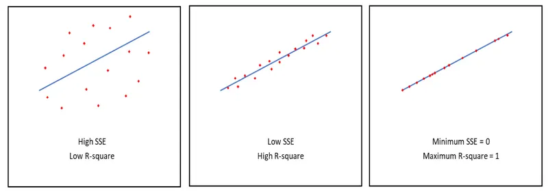
The value of R-square ranges between 0 and 1. The closer the value to 1, the better the fit.

3. Adjusted R – Square

This statistic uses the R-square statistic and adjusts it based on the residual degrees of freedom. The residual degrees of freedom is defined as the number of response values '`n`' minus the number of fitted coefficients '`m`' estimated from the response values.

`v=n-m`

' `v`' indicates the number of independent pieces of information involving the '`n`' data points that are required to calculate the sum of squares.

4. Root Mean Squared Error (RMSE)

This statistic is an estimate of the standard deviation of the random component in the data. Closer the value to 0, better the fit. It is defined by,

`RMSE = sqrt((SSE)/n`

Where, `n` = total number of datapoints available.

PROGRAM & EXPLANATION :

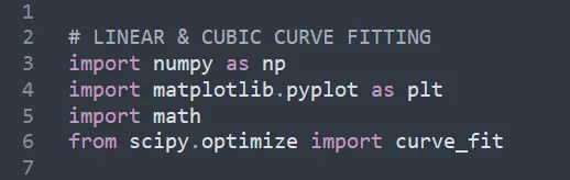
The first and foremost step in writing the programme is importing the required modules into python. Here, we import the “numpy”, “matplotlib.pyplot”, “math” and “scipy” modules.

Loading Data File :

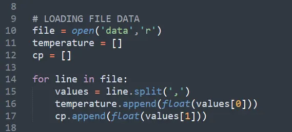
In this section, we are going to load the data file containing the specific heat values of oxygen as a function of temperature.

• The first step is opening the data file and reading the contents of it. The data file is stored in the same directory as the program and is in the form of a text file.
  
  
  
• Next, we define two empty arrays for the values of temperature and specific heat, which are going to be appended later on.
  
  
  
• The text file is then separated into 2 columns by using the ‘split’ command, which splits the data along the comma in the middle. The first column of the data is taken as temperature and the second column as the specific heat values and are further appended into their respective empty arrays.
  
  
  

Defining Curve Functions :

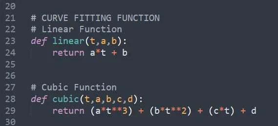
After defining our respective temperature and `C_p` arrays, we further define two functions representing the linear and cubic polynomial curves.

• The first function represents the linear polynomial equation which is of the form,
  
  `Y=ax+b`
  
  
  
• The second function represents a cubic polynomial of the form,
  
  `Y=ax^3+bx^2+cx+d`

Curve Fitting :

In this section, we are going to fit the linear and cubic polynomial functions to the original dataset.

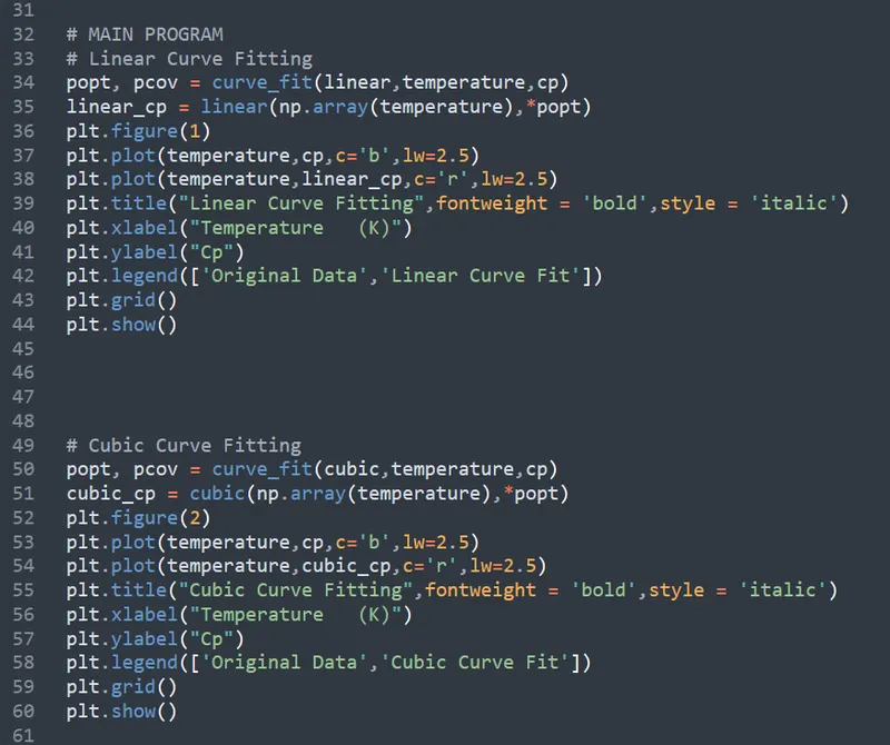
• We use the ‘curve_fit’ option, which returns two items – popt & pcov. The ‘popt’ variable provides the best-fit parameters for a, b, c & d. The ‘pcov’ variable contains the covariance matrix.
  
  
  
• From the values of popt, we calculate the predicted `C_p` values for the curve fit, with reference to the range of temperature.
  
  
  
• Finally, we plot the values of the original data set, in comparison to the calculated linear and cubic curve fits. The necessary labels and title is provided and thereby obtaining our final curve fit.

Error Calculation :

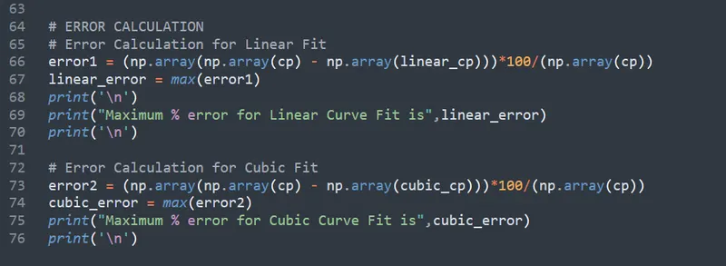
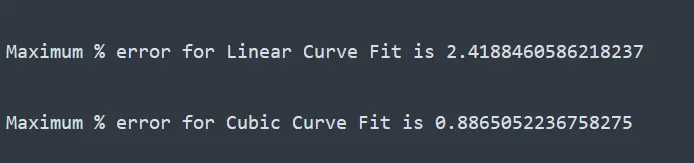
The final step in the program is to calculate the percentage error of the linear and cubic curve fits, which is a measure of the goodness of the fit.

RESULTS :

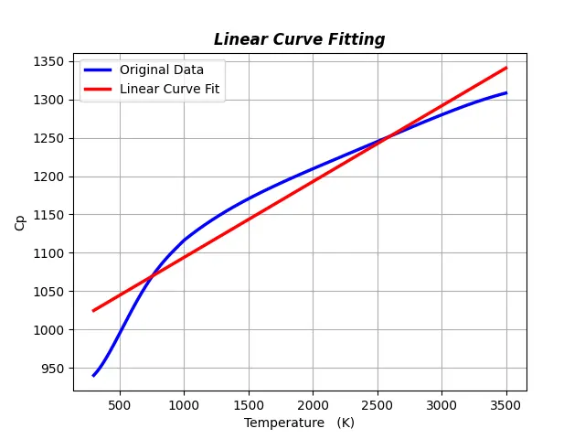
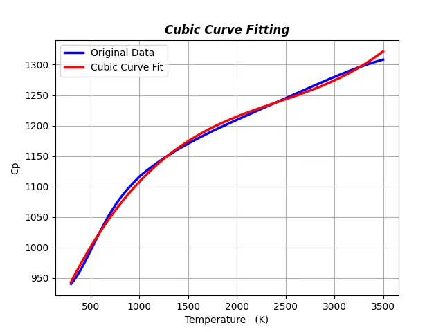
By running the above program code, we obtain the results of the linear and cubic curve fits as follows.

1. Linear Curve Fit Plot

2. Cubic Curve Fit Plot

3. Errors

The respective errors of the linear & cubic curve fits are displayed in the console as follows.

Final Program Code :

# LINEAR & CUBIC CURVE FITTING
import numpy as np
import matplotlib.pyplot as plt
import math
from scipy.optimize import curve_fit


# LOADING FILE DATA
file = open('data','r')
temperature = []
cp = []

for line in file:
	values = line.split(',')
	temperature.append(float(values[0]))
	cp.append(float(values[1]))



# CURVE FITTING FUNCTION
# Linear Function
def linear(t,a,b):
	return a*t + b


# Cubic Function
def cubic(t,a,b,c,d):
	return (a*t**3) + (b*t**2) + (c*t) + d




# MAIN PROGRAM
# Linear Curve Fitting
popt, pcov = curve_fit(linear,temperature,cp)
linear_cp = linear(np.array(temperature),*popt)
plt.figure(1)
plt.plot(temperature,cp,c='b',lw=2.5)
plt.plot(temperature,linear_cp,c='r',lw=2.5)
plt.title("Linear Curve Fitting",fontweight = 'bold',style = 'italic')
plt.xlabel("Temperature   (K)")
plt.ylabel("Cp")
plt.legend(['Original Data','Linear Curve Fit'])
plt.grid()
plt.show()




# Cubic Curve Fitting
popt, pcov = curve_fit(cubic,temperature,cp)
cubic_cp = cubic(np.array(temperature),*popt)
plt.figure(2)
plt.plot(temperature,cp,c='b',lw=2.5)
plt.plot(temperature,cubic_cp,c='r',lw=2.5)
plt.title("Cubic Curve Fitting",fontweight = 'bold',style = 'italic')
plt.xlabel("Temperature   (K)")
plt.ylabel("Cp")
plt.legend(['Original Data','Cubic Curve Fit'])
plt.grid()
plt.show()




# ERROR CALCULATION
# Error Calculation for Linear Fit
error1 = (np.array(np.array(cp) - np.array(linear_cp)))*100/(np.array(cp))
linear_error = max(error1)
print('\n')
print("Maximum % error for Linear Curve Fit is",linear_error)
print('\n')

# Error Calculation for Cubic Fit
error2 = (np.array(np.array(cp) - np.array(cubic_cp)))*100/(np.array(cp))
cubic_error = max(error2)
print("Maximum % error for Cubic Curve Fit is",cubic_error)
print('\n')

Q1.) What does ‘popt’ and ‘pcov’ mean?

• The return value ‘popt’contains the best-fit values (optimal values) of the parameters.
  
  
• The return value ‘pcov’contains the covariance (error) matrix for the fit parameters. From them we can determine the standard deviations of the parameters.

Q2.) What does ‘np.array(temperature)’ do?

This command converts each and every value of temperature in the data file into an array, by using the numpy module.

Q3.) What does the * in ‘*popt’ mean?

The star in *popt unpacks the popt array so the two optimized parameter values become the second and third arguments to the function.

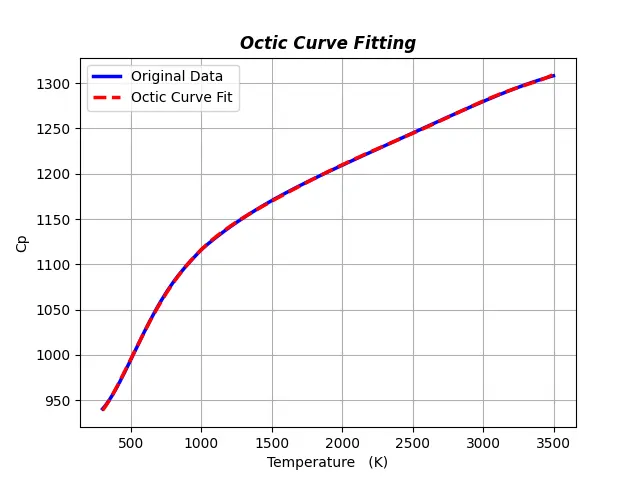
Q4.) What needs to be done in order to make the curve fit perfect?

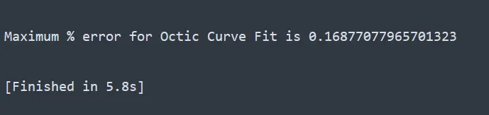
In order to get a perfect fit, the value of R - Square must be exactly equal to 1. This can be achieved by increasing the degree of the polynomial.

By raising the degree of the polynomial to 8 (octic polynomial), we get a better quality of curve fit as compared to the linear and cubic curve fits.

CONCLUSIONS :

A Python program representing a linear & cubic polynomial fit over the given data of specific heat values of oxygen as a function of temperature has been successfully written and the following outputs have been obtained as shown above.

From the results, we can observe that as the degree of the polynomial increases, the quality of the curve fit gets better as well. Therefore, higher the degree of the polynomial, better the curve fit.

Thereby, we can conclude that in order to obtain a perfect fit, the value of R-square must be nearer to 1.