Week 6 - CHT Analysis on a Graphics card
AIM :
To perform a steady-state conjugate heat transfer analysis on the model of a graphics card.
OBJECTIVES :
- Carry out the simulation by varying the velocity from 1 m/sec to 5 m/sec for at least 3 velocities and discuss the results.
- Run the simulation for best possible mesh with combination of coarse and refined mesh in different regions. Explain the reason for choosing the particular mesh settings.
- Find out the maximum temperature and heat transfer coefficient attained by the processor, by using the appropriate materials of your choice for the simulation.
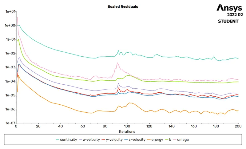
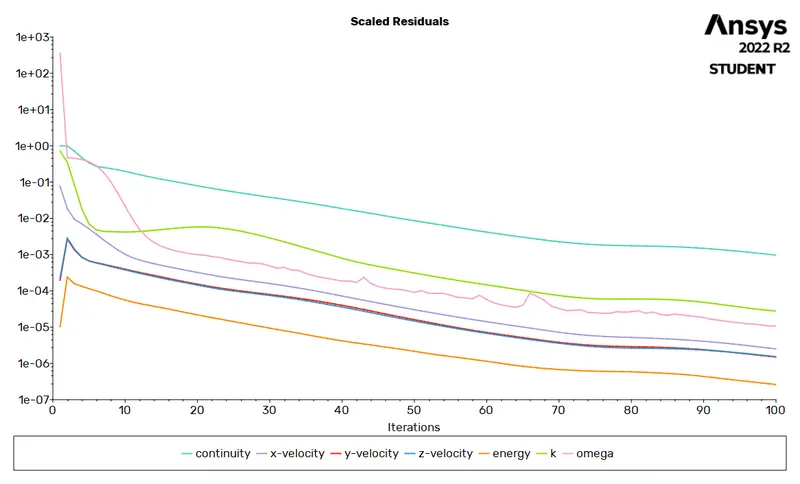
- Prove that the simulation has achieved convergence with appropriate images and plots.
- Identify potential hotspots on the model.
INTRODUCTION :
Graphics cards can use the same power as that of a 150 Watt lamp. With so much power running through today's integrated circuits, the internal thermal resistance from the flow of electricity creates enormous amounts of heat. This heat can damage these devices if they are not properly cooled.
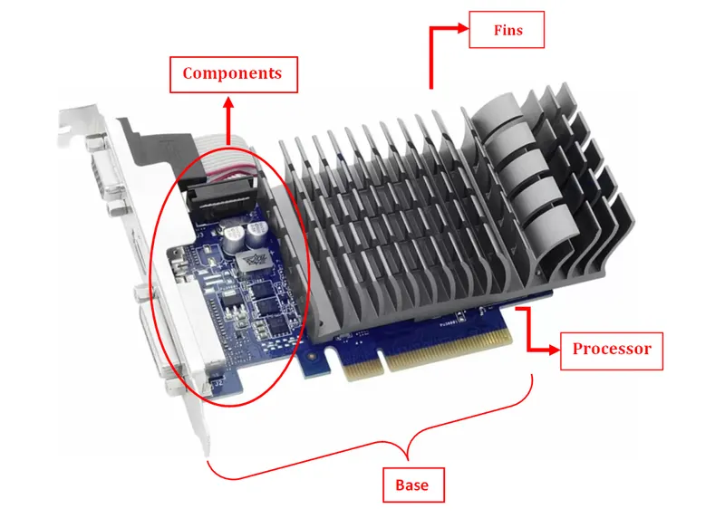
All graphics cards have an ideal temperature range for operation. Under normal conditions, only the upper limit really ever becomes relevant. Exceeding that temperature causes a decrease in performance and can eventually cause the card permanent heat damage.
Conjugate heat transfer :
Conjugate heat transfer is a type of heat transfer analysis between solids and fluids. This type of heat transfer includes both convection (between fluids) and conductive (between solids) heat transfer, as well as both forced and natural convection. Common applications and use cases of this thermal simulation type include electronics cooling, heat exchangers, industrial machinery, heaters, some AEC cases, and more.
Heat Transfer Co-Efficient :
Heat transfer co-efficient defines the rate of heat transfer between a solid surface and a fluid per unit surface area per unit temperature difference. It refers to how well heat is conducted through a series of resistant mediums.
The general formula of the heat transfer coefficient is:
`h=q/(DeltaT)`
Where,
`q` = Local heat flux density (`W`/ `m^2`)
`h` = Heat transfer coefficient (`W`/`m^2⋅K`)
`DeltaT` = Temperature difference (`K`)
CASE SETUP :
For this simulation, we set up 3 case studies. The first case study represents the mesh dependency test, wherein we are going to setup 2 sub-cases for the coarse mesh and refined mesh respectively, and study the effect of meshing element size on the simulation results. In the next 2 cases, we are going to increase the air inlet velocity and study the effects of cooling obtained.
The case setup along with the details and materials used is as represented below.
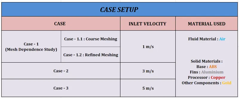
SIMULATION PROCEDURE :
For this simulation, we are going to setup the Fluid Flow (Fluent) module in ANSYS Workbench to carry out the simulation in 5 steps namely,
- Geometry
- Meshing
- Setup
- Solution
- Results
General Setup :
The general ANSYS Workbench setup stage is the same for all the 3 cases and is as follows.
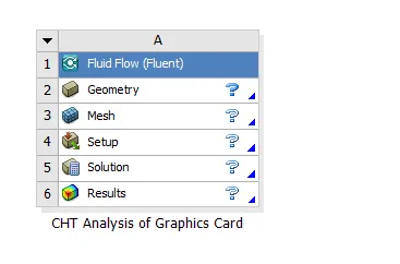
The first and foremost step in running the simulation is importing the geometry of the graphics card into the ANSYS SpaceClaim software and identifying each individual part of the geometry. The various components of the geometry are as shown below.
1. BASE
The base is basically a support system, on which all the components of the graphics card, such as capacitors, processors and transistors are mounted on. It also contains the input and output ports as well. It is usually made up of a light-weight plastic such as silicon or fibreglass.
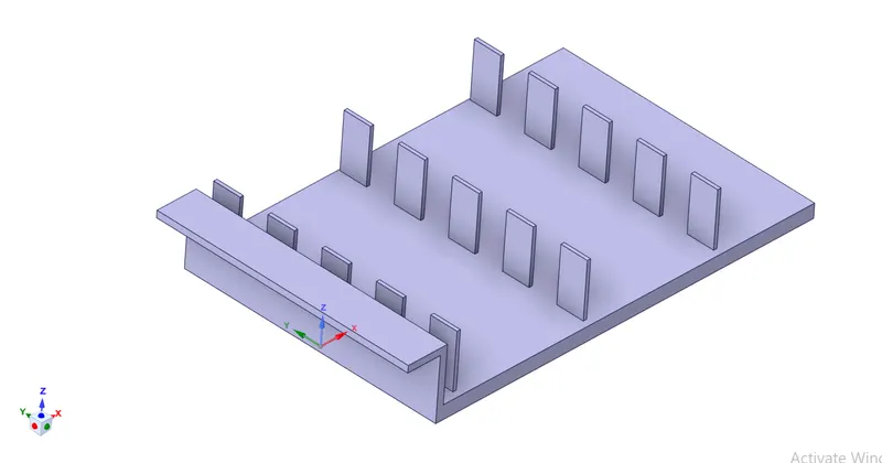
2. FINS
The main function of the fins is to maintain optimal operating temperature of the processor. The heat generated by the processor is conducted to the fins, which has a larger surface area as compared to the processor. Heat is dissipated across the fins, and when air is passed through it, heat transfer takes place through convection. This thereby leads to more efficient cooling and the processor is maintained at the optimal temperature range.
3. PROCESSOR
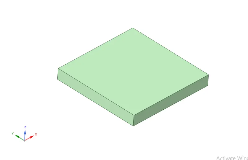
The processor is a chip placed in the motherboard, which is responsible for millions of processes that, in combination with other components, makes the whole device run. Processors constantly send information through electrical signals. This electricity running over the circuit generates heat. And while this is completely normal, an excessively higher temperature may damage the processor. Hence, cooling the processor and maintaining it at an optimal temperature becomes necessary.
4. ENCLOSURE
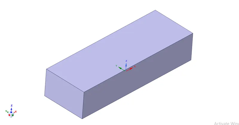
The enclosure inside which the graphics card is nested in, acts as a domain, which we use to simulate the air flow and study its characteristics.
CASE – 1 : MESH DEPENDENCE TEST (Inlet Velocity = 1 m/s)
For this particular case study, we are going to setup 2 sub-cases. One being a case study for a coarse meshing and the other for a refined mesh case, so as to compare the results.
Case 1.1 : Coarse Meshing
The processes involved in carrying out the simulation is as follows.
1. GEOMETRY
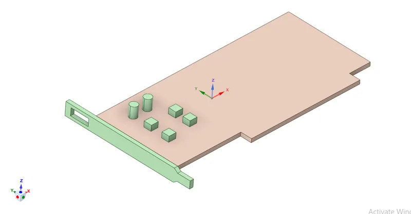
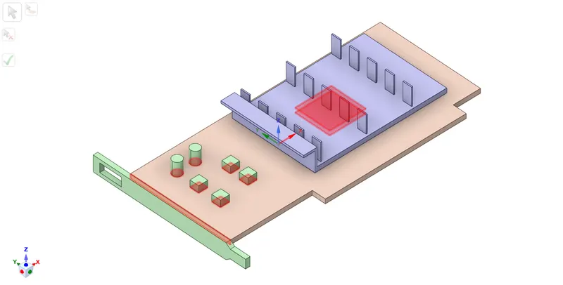
In this step, we first import the provided step file into the ANSYS SpaceClaim software. The geometry of the graphics card, including all the components is as shown.
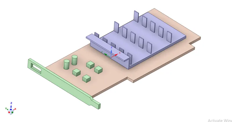
Next, we make sure the share topology of the geometry is enabled, so as to obtain conformal meshing. We do this using the “share” function, which shares the coincident topology.
Thereby, we share a total of 9 faces and 32 edges.
2. MESHING
In this step, we generate the base mesh for the geometry as shown below.
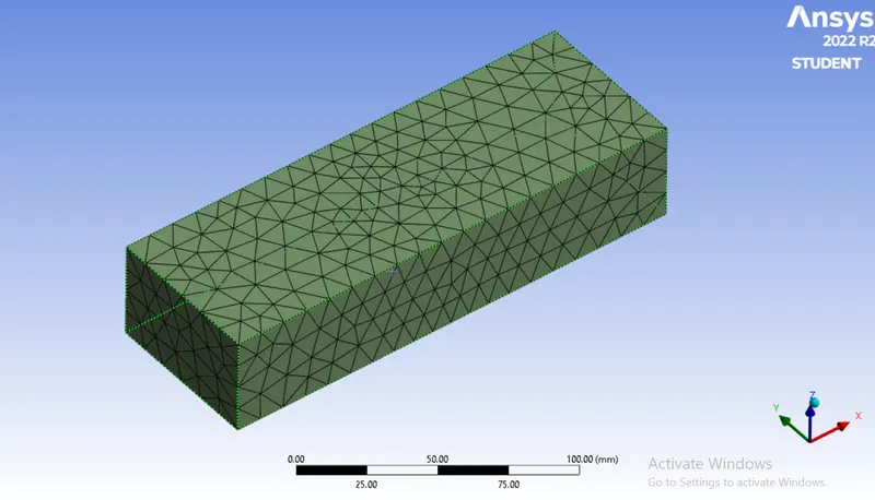
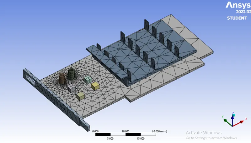
We create a cut-plane to obtain the cross-sectional view of the meshed geometry.
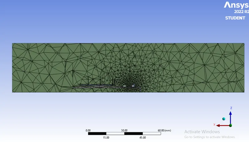
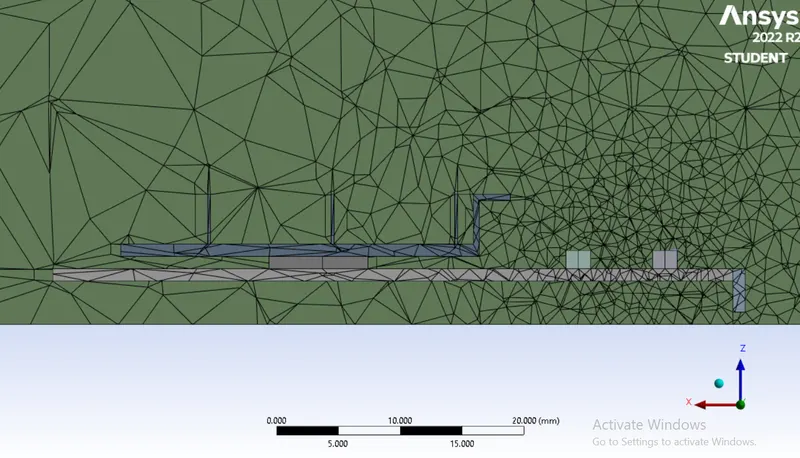
Next, we create named selections of the respective components and the boundary conditions of the graphics card as well as the enclosure. The created named selections are as follows.
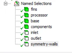
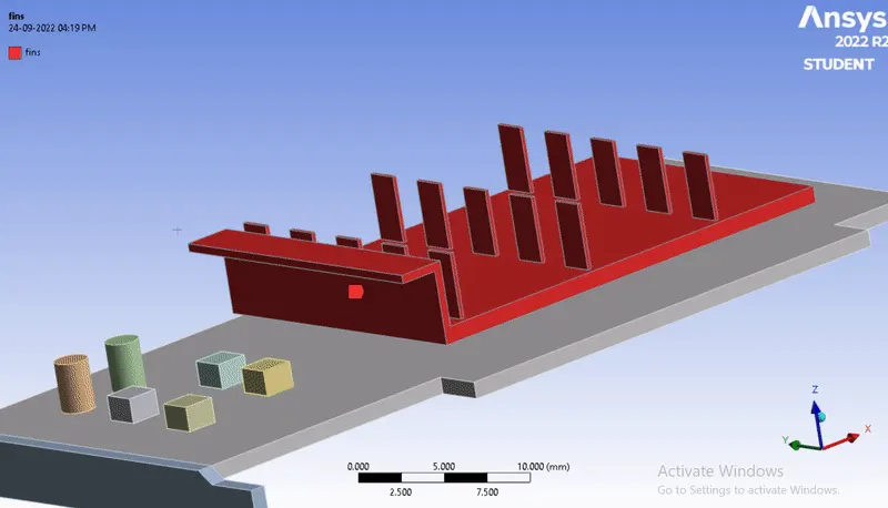
3. SETUP & SOLUTION :
In this step, we setup the necessary conditions to run the simulation in ANSYS Fluent.
We use a pressure – based steady state solver with absolute velocity formulation to run the simulation.
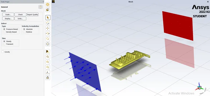
- We activate the energy equation, which enables us to obtain the temperature of the fluid involved in heat transfer.
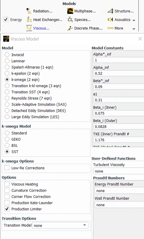
- We use the k – omega SST turbulence model in this case, as it is the best for near – wall treatment. The SST model provides a better prediction of flow separation.
The next step in the simulation setup is the material selection. We setup the following materials from the Fluent Database.
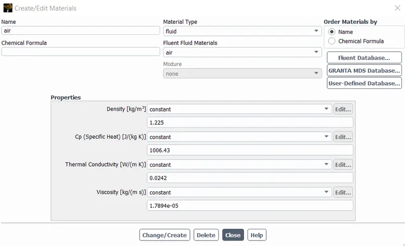
FLUID MATERIAL (Air) :
We use air as the surrounding fluid medium inside the domain (enclosure).
SOLID MATERIALS :
We allot different materials to the different components of the graphics card as shown below.
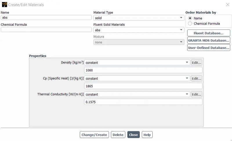
1. Acrylonitrile Butadiene Styrene (ABS)
The material of the base of the graphics card is taken to be ABS, due to its high rigidity and good insulating properties.
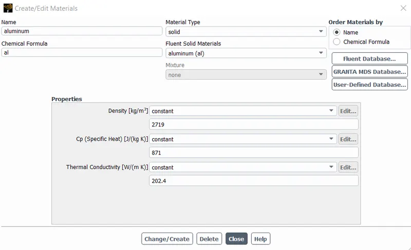
2. Aluminium (Al)
The material of the fins is considered as aluminium, as it dissipates the heat effectively due to its high thermal conductivity properties.
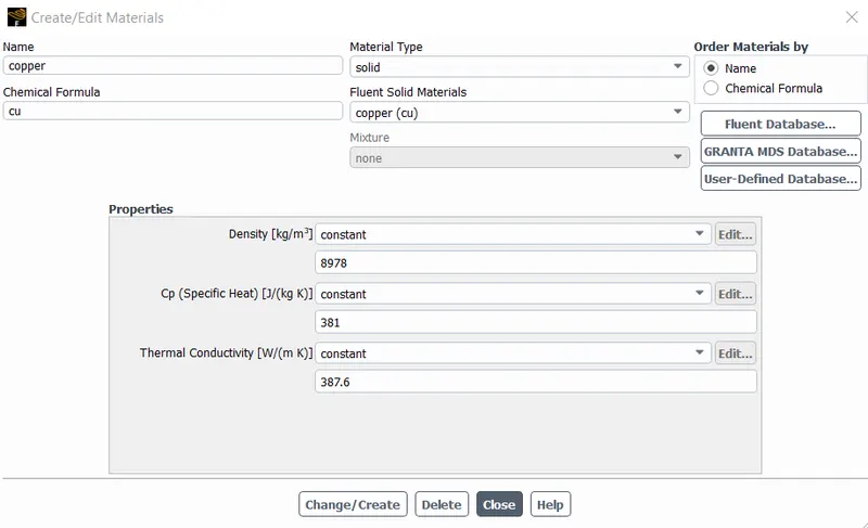
3. Copper (Cu)
The processor is considered to be made copper, as it is a good conductor of heat.
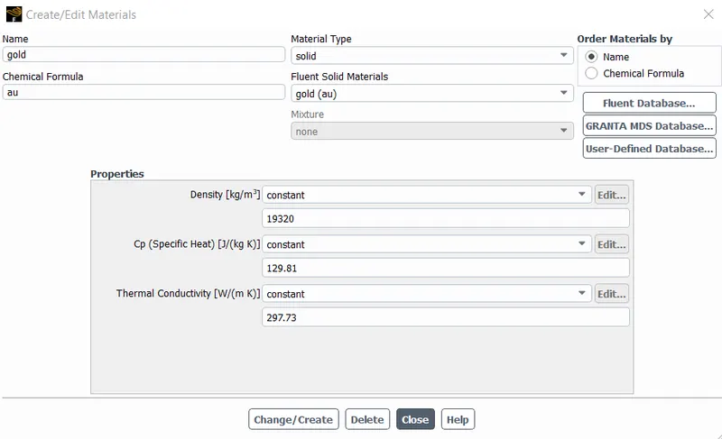
4. Gold (Au)
All the other components of the graphics are considered to be of gold.
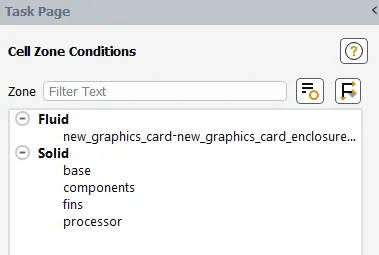
The components and the materials are classified into two categories of cell-zones, on basis of the material, as shown below.
As electrons move through wires, it produces heat. On a small computer chip, the area to dissipate heat isn’t very much and is concentrated. Thus, it heats up to high temperature. This makes the processor, the main source of heat in the graphics card.
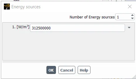
To simulate this generated heat, we enable the source term for the processor in which we enter the energy source value.
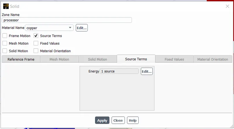
The processors in desktop computers use between 30 and 90 watts. To calculate the energy source value of the processor, we consider the processor is operating at a power consumption range of 20 watts.
Power Consumption (`P`) = `20` `W`
Volume of the Processor (`V`) = `64` `mm^3`
As we know,
`"Heat Generated" = P/V` `= 20 / (64 xx 10^-9)`
`therefore` Heat Generated = 312500000 `W`/`m^3`
- Finally, before running the calculations, we setup the inlet velocity boundary conditions as 1 m/s and also the outlet pressure condition as 0 gauge pressure.
- We also define the reports so as to obtain the plots of maximum temperature achieved by the processor and the wall heat transfer co-efficient of the geometry.
- The temperature contours along with the solution animations are also setup after initialization (standard).
- We run the simulation for 200 iterations to obtain the following results.
4. RESULTS
By running the simulation with the above mentioned setup conditions, we obtain the following results.
Residuals Plot :
Temperature Plots :
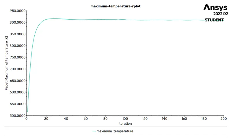
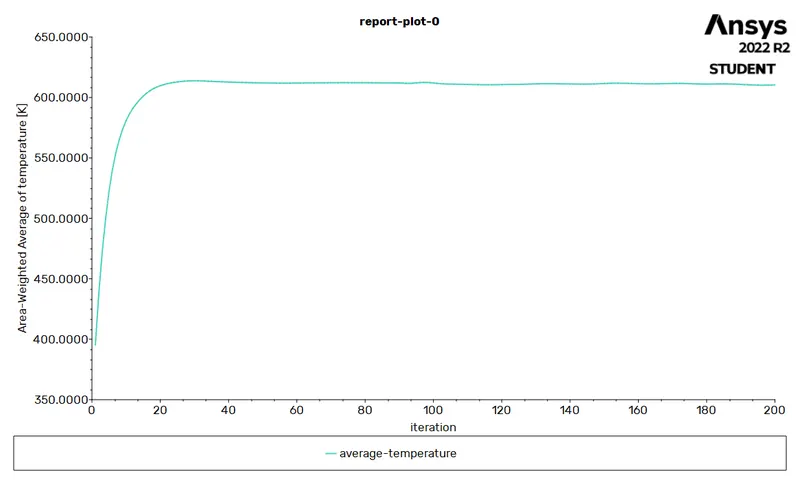
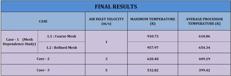
From the above plots, we can observe that the average wall temperature is 610.86 K and the maximum temperature achieved by the processor is 910.73 K.
Temperature Contour Plot :
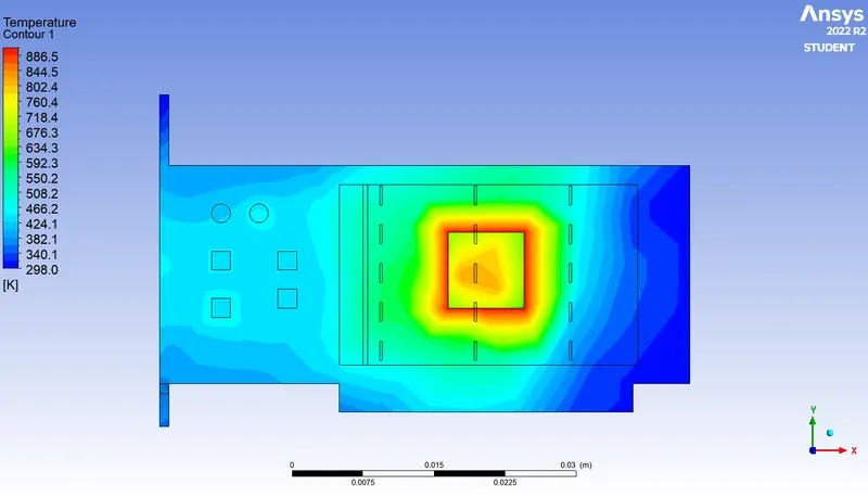
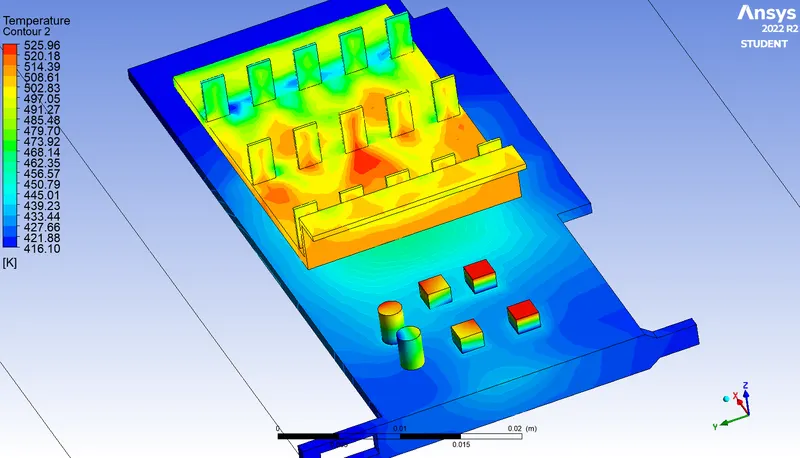
The temperature distribution across the graphics card, with the processor being the main source of heat, is as shown above.
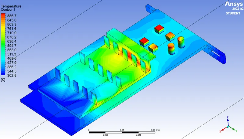
The local temperature contour of the card is as shown.
Velocity Profile :
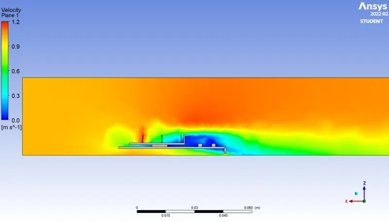
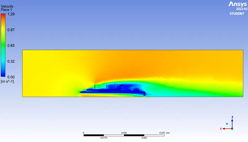
We can observe that the velocity profile is pretty distorted, which is due to the coarse (baseline) meshing.
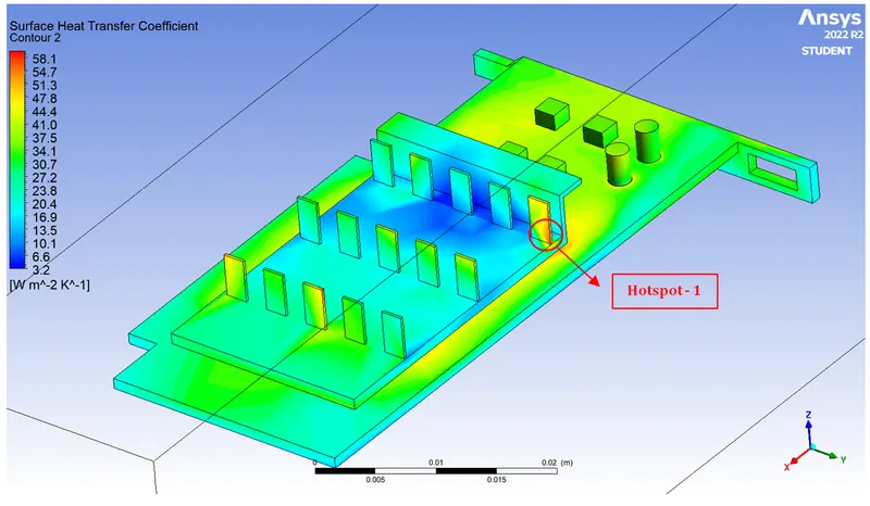
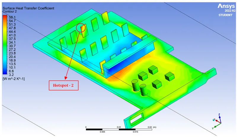
Wall Heat-Transfer Co-efficient :
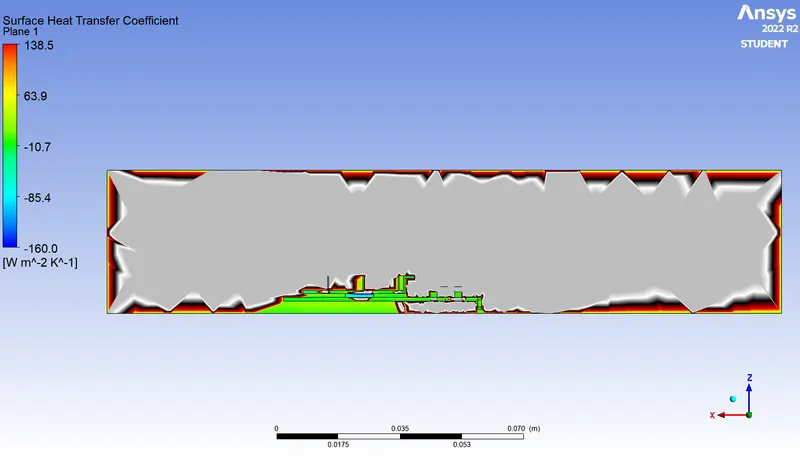
Maximum Heat Transfer Co-efficient Regions :
Case 1.2 : Refined Meshing
For this case study, we refine the meshing for the same geometry, by adding inflation layers and face sizing parameters.
To refine the mesh, we first create a body sizing of element size 3 mm, of the outer enclosure.
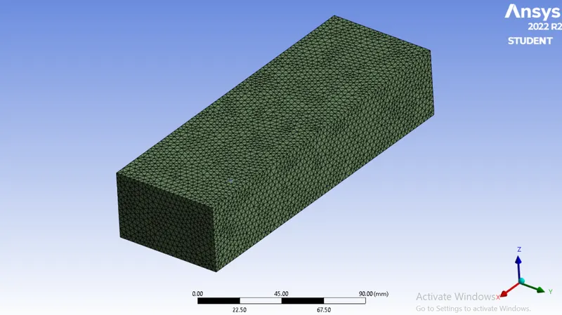
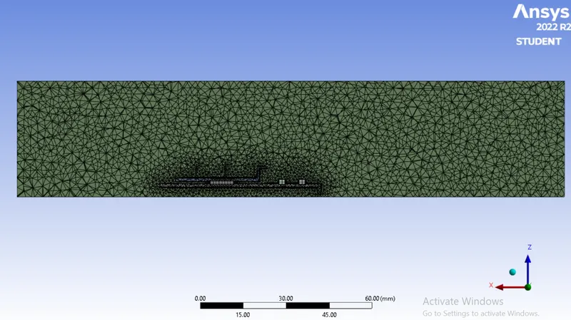
As most of the flow separation occurs around the graphics card, we need to capture these details accurately. Therefore, we refine the mesh around the graphics card area, so as to accurately capture the flow variations. This refining is achieved by face sizing, to an element size of 1 mm.
Also, we create 5 inflation layers around the side – wall boundary of the graphics card, with a total thickness of 0.4 mm.
Face Sizing :
Inflation Layer :
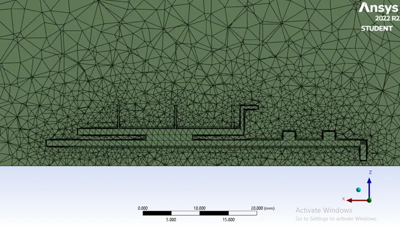
Finally, to accurately capture the temperature distribution and air flow over the fins, we create face sizing, of an element size of 2 mm, so as to obtain a refined meshing.
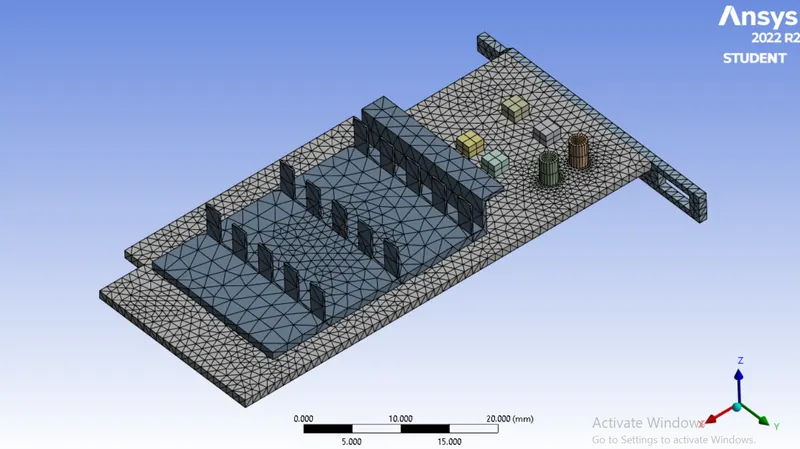
For the same Fluent setup, we carry out the simulation of the refined mesh for an inlet velocity of 1 m/s. We run the simulation for 100 iterations and thereby obtaining the following results.
Residuals Plot :
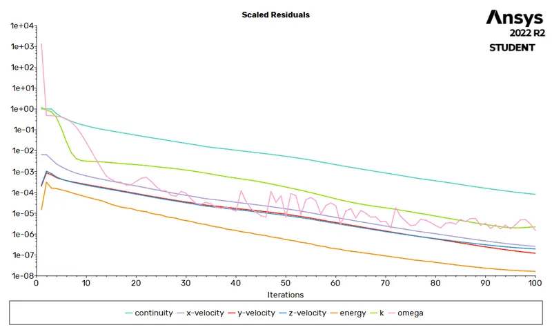
For this particular simulation, convergence is achieved at around 65 iterations but we run the simulation further.
Temperature Plots :
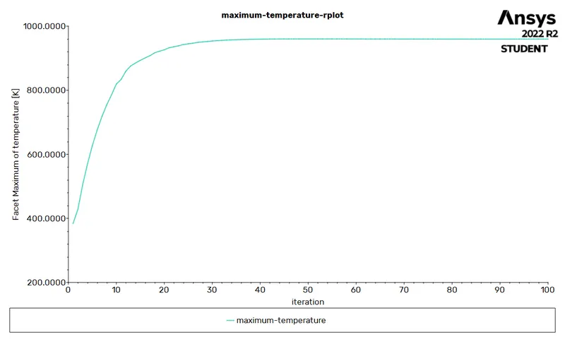
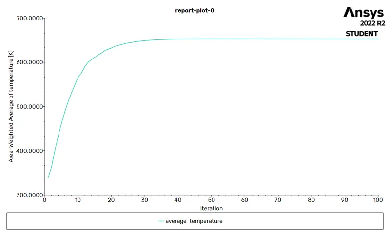
From the above plots, we can observe that the average wall temperature is 654.34 K and the maximum temperature achieved by the processor is 957.97 K.
Temperature Contour Plot :
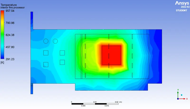
The temperature distribution across the graphics card, with the processor being the main source of heat, is as shown above.
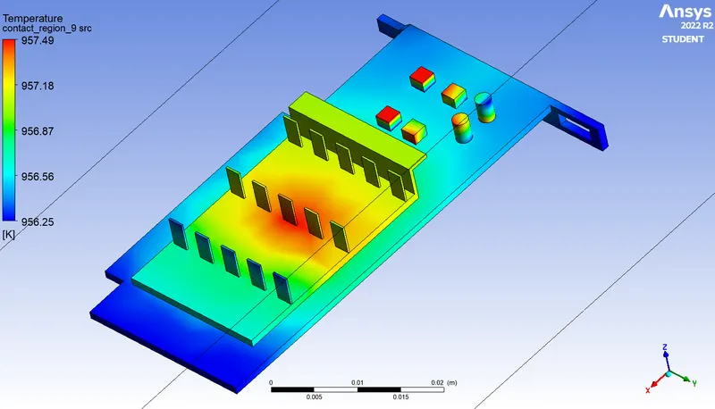
The local temperature contour of the card is as shown.
Velocity Profile :
Wall Heat-Transfer Co-efficient :
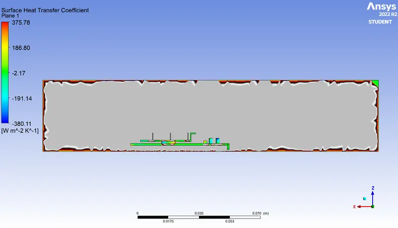
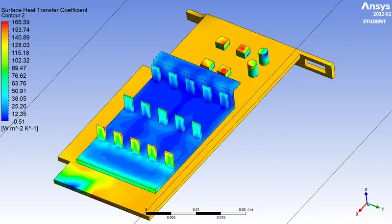
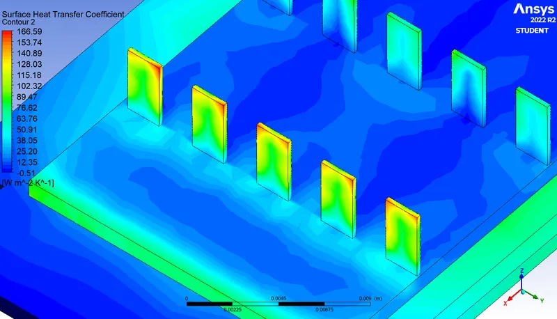
Maximum Heat Transfer Co-efficient Regions :
CASE – 2 : INLET VELOCITY = 3 m/s (Refined Mesh)
The benchmark parameters of the simulation setup are as follows.
Geometry
Share Topology : ON
Meshing
Meshing Element Size : 5 mm
Face Sizing : 1 mm
Inflation Layers : 5 layers of 0.4 mm total thickness
Setup
Solver : Pressure – based
Velocity Formulation : Absolute
Time Management : Steady state
Energy Equation : ON
Turbulence Model : k – omega SST
Materials : Fluid `->` Air (enclosure)
Solid `->` ABS (base)
Aluminum (fins)
Gold (components)
Copper (processor)
Energy Source Term : 312500000 `W`/`m^3` (processor)
Inlet Velocity : 3 `m`/`s`
Outlet Pressure : 0 gauge (1 atm)
Solution
Initialization : Standard
Iterations : 100
We run the simulation for the above mentioned parameters to obtain the following results.
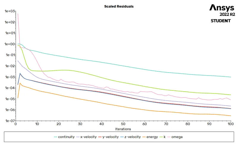
Residuals Plot :
Temperature Plots :
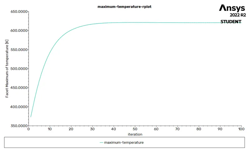
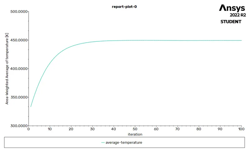
From the above plots, we can observe that the average wall temperature is 449.19 K and the maximum temperature achieved by the processor is 620.48 K.
Temperature Contour Plot :
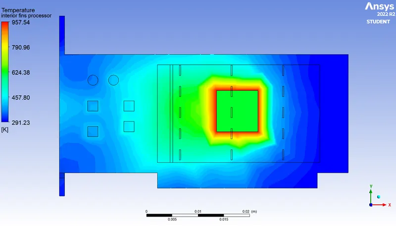
The temperature distribution across the graphics card is as shown above.
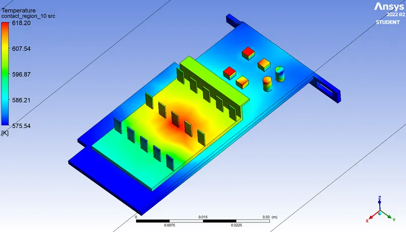
The local temperature contour of the card is as shown.
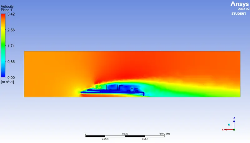
Velocity Profile :
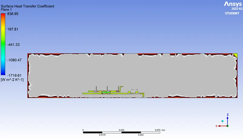
Wall Heat-Transfer Co-efficient :
Maximum Heat Transfer Co-efficient Regions :
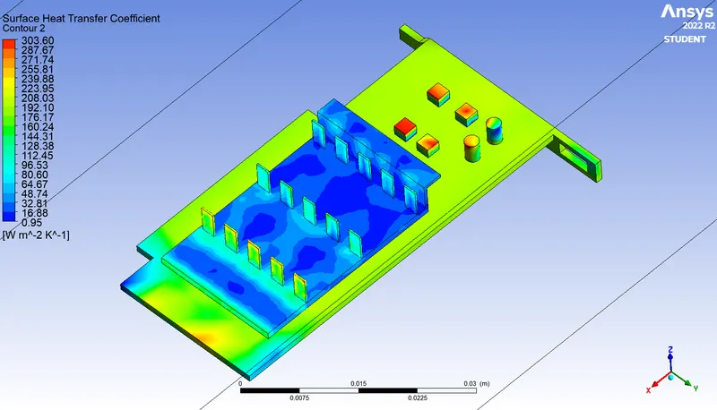
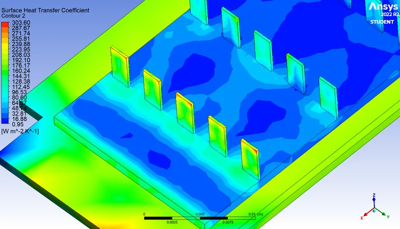
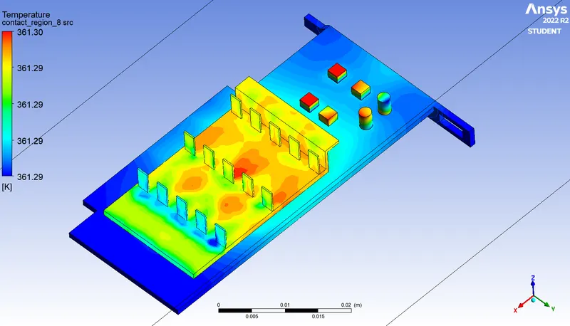
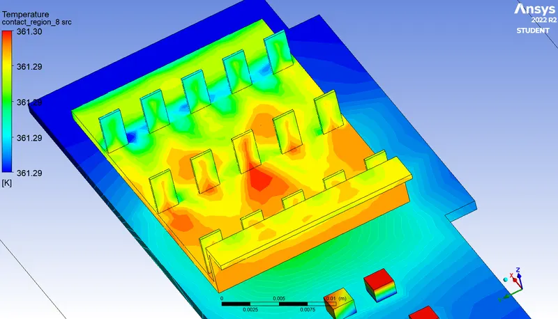
Potential Hotspot Regions :
CASE – 3 : INLET VELOCITY = 5 m/s (Refined Mesh)
The benchmark parameters of the simulation setup are as follows.
Geometry
Share Topology : ON
Meshing
Meshing Element Size : 5 mm
Face Sizing : 1 mm
Inflation Layers : 5 layers of 0.4 mm total thickness
Setup
Solver : Pressure – based
Velocity Formulation : Absolute
Time Management : Steady state
Energy Equation : ON
Turbulence Model : k – omega SST
Materials : Fluid `->` Air (enclosure)
Solid `->` ABS (base)
Aluminum (fins)
Gold (components)
Copper (processor)
Energy Source Term : 312500000 `W`/`m^3` (processor)
Inlet Velocity : 5 `m`/`s`
Outlet Pressure : 0 gauge (1 atm)
Solution
Initialization : Standard
Iterations : 100
We run the simulation for the above mentioned parameters to obtain the following results.
Residuals Plot :
Temperature Plots :
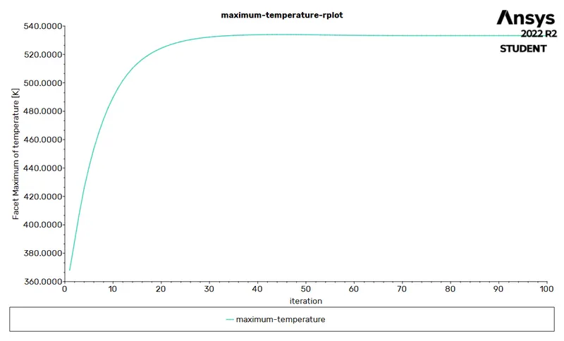
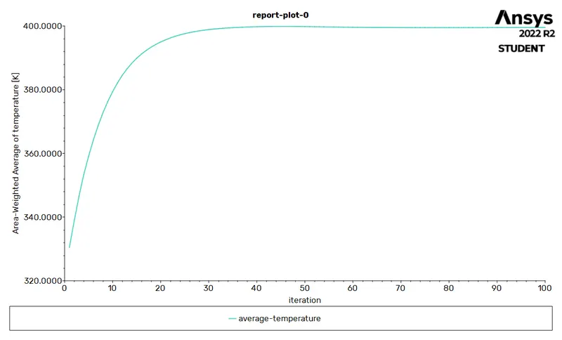
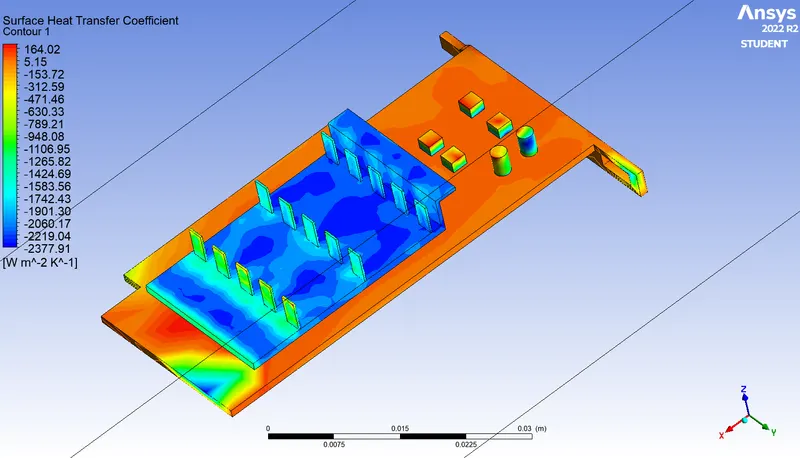
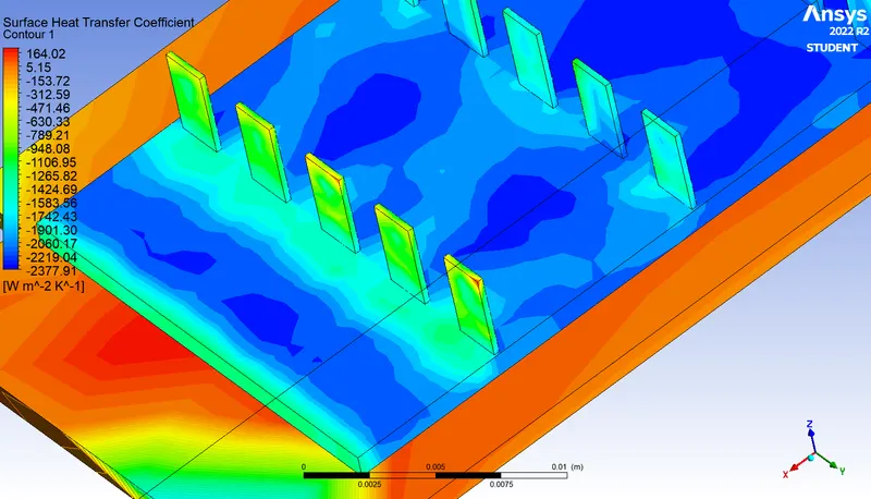
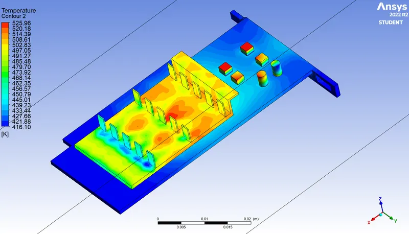
From the above plots, we can observe that the average wall temperature is 399.42 K and the maximum temperature achieved by the processor is 532.82 K.
Temperature Contour Plot :
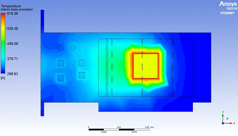
The temperature distribution across the graphics card is as shown above.
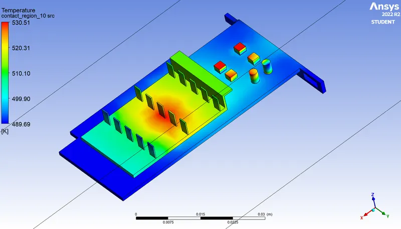
The local temperature contour of the card is as shown.
Velocity Profile :
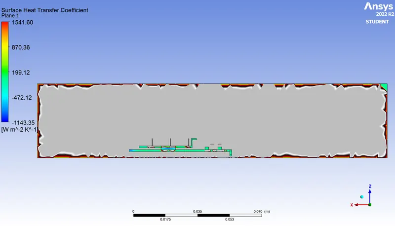
Wall Heat-Transfer Co-efficient :
Maximum Heat Transfer Co-efficient Regions :
Potential Hotspot Regions :
FINAL RESULTS :
By running the simulation for the respective number of iterations and various inlet velocities, we obtain the following results.
CONCLUSIONS :
The simulation has been successfully carried out for all 3 case studies and the respective plots and contours have been obtained, as shown.
From the above results, we can observe that, with increase in the number of elements of meshing and by adding inflation layers and face sizing around the area of interest, i.e., by refining the mesh, we obtain much more accurate and well defined results as compared to the coarse or baseline mesh. The details of flow separation of air around the graphics card geometry are captured in detail, by a refined mesh. Therefore, the mesh refinement plays an important role in the accuracy of the simulations.
The processor is considered to be the main heat source of the graphics card, which in operation, produces a lot of heat. We have carried out 3 case studies wherein we have increased the air inlet velocity to study the effects of cooling. Here, we can observe from the cases that, as we increase the inlet flow velocity of air, it thereby leads to a reduce in the temperature of the processor. Thereby, an increase in inlet flow velocity leads to more efficient cooling of the processor. The processor can be maintained at optimal temperature by increasing the inlet velocity of air, thereby reducing the chances of damage.
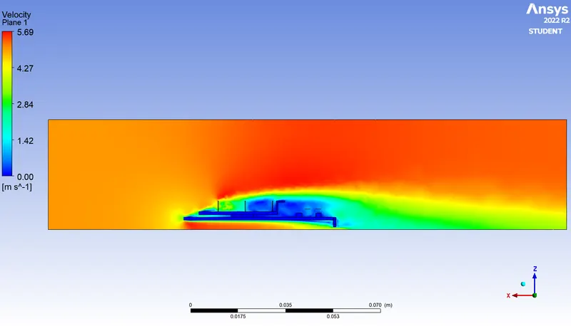
As we know, the heat transfer coefficient expresses the amount of heat transferred between a fluid and a solid surface by convection. The larger the heat transfer coefficient, the more heat transfer occurs. Another factor that greatly influences the magnitude of the heat transfer coefficient is the fluid flow velocity over the object surface. Therefore, higher the inlet velocity, the larger the heat transfer coefficient.