Week 7 - Simulating Fluid Sloshing effect inside a Gear-box

AIM :

To simulate the fluid sloshing effect inside the gearbox for different levels of immersion of engine oil and n – heptane (C7H16).

INTRODUCTION :

A Gear Box is often called a transmission. Gear boxes simply refer to a set of gears and their casing. Gearboxes are used to transfer energy from one rotating power source to another and can be found in automobiles, turbines, and heavy machinery.

The gears inside of a gearbox can be any one of a number of types from bevel gears and spur gears to worm gears and others such as planetary gears. The gears are mounted on shafts, which are supported and rotate via rolling element bearings. The gearbox is a mechanical method of transferring energy from one device to another and is used to increase torque while reducing speed.

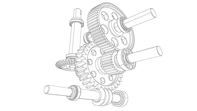
What does the gearbox do?

• Acceleration and deceleration, which are often referred to as speed change gearboxes.
• Changing the transmission direction, such as using two sector gears to transmit the force vertically to the other rotating shaft.
• Changing torque: Under the same power conditions, the faster the gear rotates, the smaller the torque on the shaft, and vice versa.
• Clutch function: The purpose of separating the engine from the load can be achieved by separating the two originally meshed gears. such as brakes, etc.
• Distribute power: For example, one engine can be used to drive multiple slave shafts through the main shaft of the gearbox, to realize the function of one engine driving multiple loads.

Why is lubrication necessary?

Lubrication is a crucial element in the efficiency and life-expectancy of any rotating equipment. Gearboxes rely on lubrication to reduce friction and provide cooling for optimal operation and life. Gearbox manufacturers provide recommendations for the type of lubrication to be used and the typical lubrication intervals, but the actual gearbox lubrication requirements depend on the environmental conditions the gearbox is exposed to, whether it is properly maintained, and whether it experiences overloading.

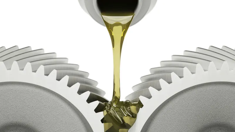
There are several methods for lubricating a gearbox, with the most common being grease lubrication, oil splash and forced oil lubrication.

Application Fields of Gearboxes :

Widely used in printing and packaging machinery, three-dimensional garage equipment, environmental protection machinery, conveying equipment, chemical equipment, metallurgical mining equipment, steel power equipment, mixing equipment, road construction machinery, sugar industry, wind power generation, escalator elevator drive, shipbuilding, light industry field, papermaking field, metallurgical industry, sewage treatment, building material industry, hoisting machinery, conveyor line, assembly line, etc. Relevant high power, high-speed ratio, high torque occasions.

CASE SETUP :

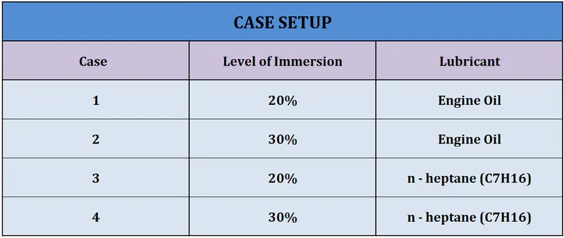
For this challenge we are running 4 cases of gearbox simulations with two different levels of immersion and with the two different fluids, so as to observe the flow patterns of the fluid inside the gearbox.

PART – 1 : SIMULATION

In this section, we carry out the simulation to observe the flow characteristics of the fluid sloshing inside the gearbox, for all 4 of the above mentioned case studies. We first setup the simulation as follows.

General Setup :

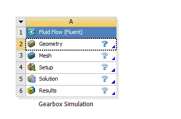
The general setup of the simulation is the same for all 4 cases. We carry out the simulation in ANSYS Workbench, in 5 steps, namely.

1. Geometry
2. Meshing
3. Setup
4. Solution
5. Results

Geometry Preparation :

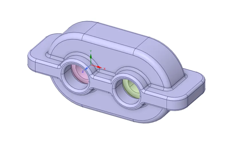
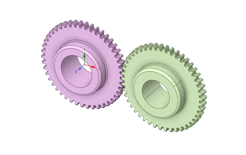
The first step in setting up the simulation involves the preparation of the geometry. We first import the provided step file of the geometry into the ANSYS SpaceClaim software. The gearbox geometry consists of two external spur gears with their teeth inter-meshed with each other and both of which are enclosed in a casing or a housing.

The external housing of the gearbox geometry is as follows.

The two spur gears which are enclosed inside the housing are as shown.

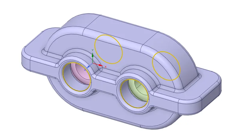
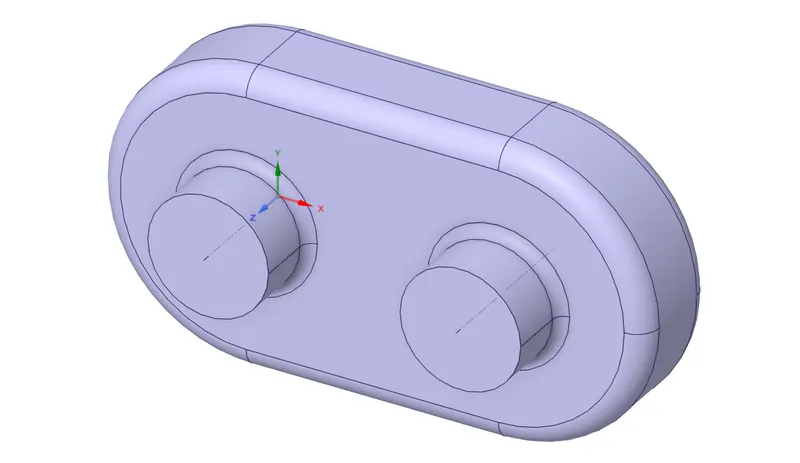
In the next step of the geometry setup, we perform volume extraction, so as to extract the fluid volume of the geometry. We do this by using the volume extract function, wherein we select the edges of the inlet and outlet regions of the fluid.

The fluid volume extraction of the geometry is obtained as,

After obtaining the volume extract, we then split the body in half by using the “split body” function. To do this, we first create 3 planes normal to the x, y and z – axes, with respect to the origin. Next, by selecting the volume extract as the target body, we obtain a split body geometry as follows.

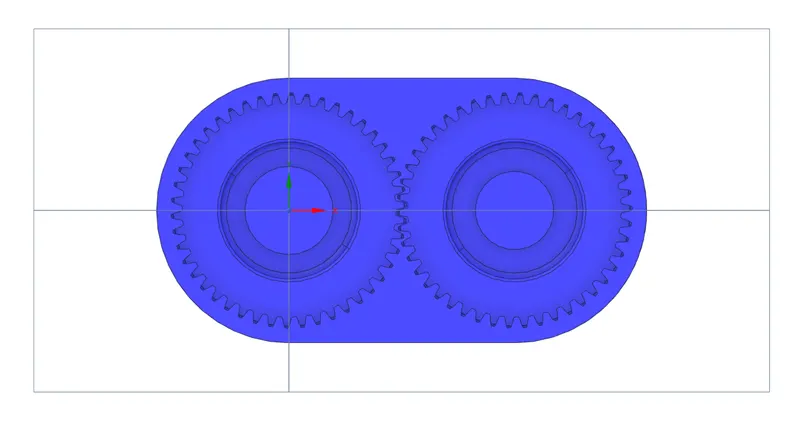
We split the body in half so that we can extract a 2 – D surface from the geometry, on which we carry out the analysis. To do so, we copy the highlighted region of the geometry as shown below and copy it onto a new plane (XY plane).

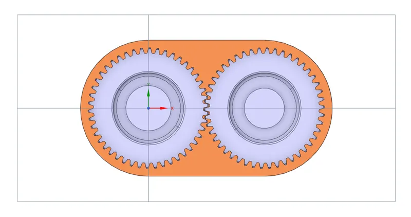
The final 2 – D geometry of the geometry is obtained as follows.

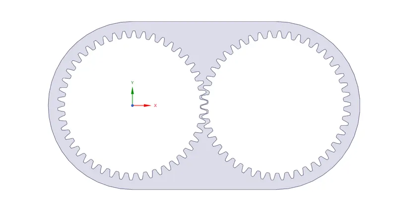
As a final step, we calculate the percentage levels of immersion of the fluid, for the 2-D geometry. The level of immersion refers to the extent to which the fluid or lubricant is filled up, when the gears are not in a running state.

From the diagram, it can be noted that the total height of the gearbox is 135 mm. Thereby, calculating the immersion levels based on this height, we get.

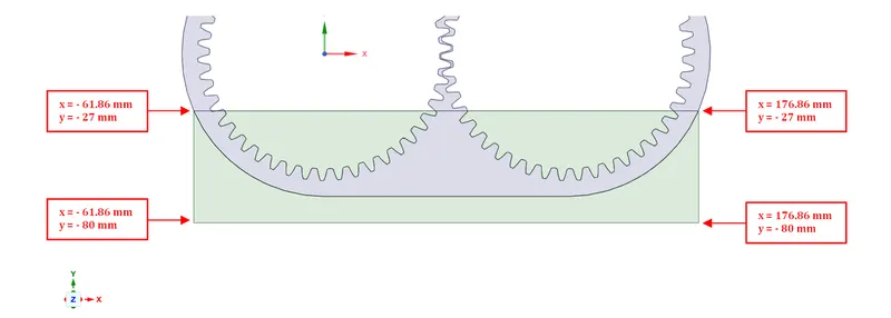
20% immersion = `0.2×135` = `27` `"mm"` from base

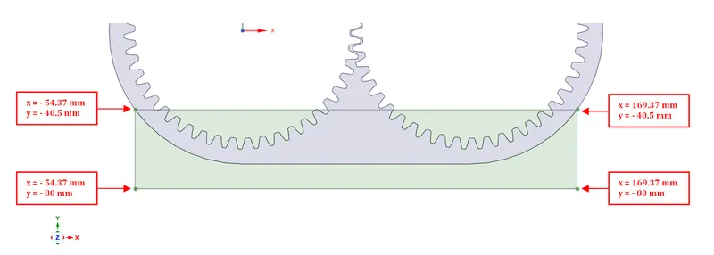
30% immersion = `0.3×135` = `40.5` `"mm"` from base.

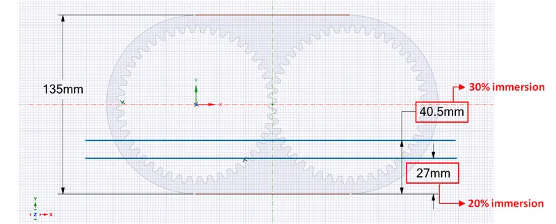
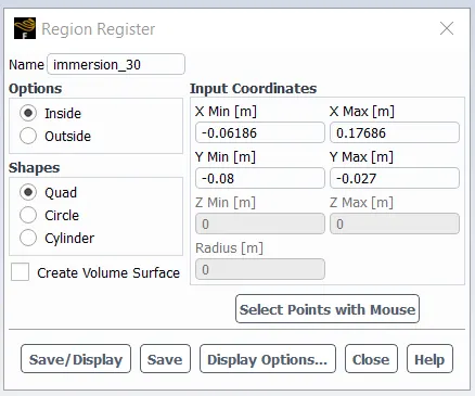
For the different immersion levels calculated above, we note down the co-ordinates of the points enclosing the region of immersion as follows.

20% immersion level :

30% immersion level :

The distance between the centroids of the gears is 115 mm. So its co-ordinates are taken as (115 , 0 , 0).

Meshing :

In this step, we generate the meshing for the obtained 2-D geometry. To do so, we first create named selections of the left gear and right gear respectively.

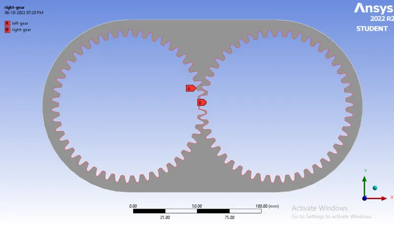
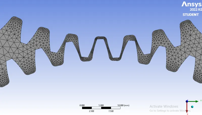
Next, we generate a triangular mesh of element size 20 mm by using the “methods” function. We obtain the meshed geometry as follows.

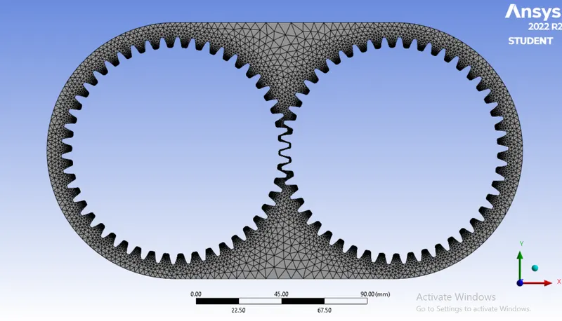
Also, we enable the “capture proximity” command so as to capture the small gaps at the intersection of the mating teeth and thereby obtaining a more accurate mesh.

Simulation Setup :

To setup the simulation and solver requirements, we first import the meshed geometry model into ANSYS Fluent.

Benchmark Parameters :

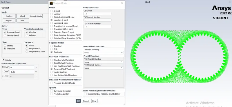
• We use a pressure – based solver with absolute velocity formulation for this simulation, which is traditionally used for incompressible and mildly compressible flows.
• We use a transient time management condition, so as to capture the flow patterns of the fluid at each and every timestep.
• We enable the gravitational effect acting along the negative y – axis, at a value of 81 m/s.
• For this simulation, we use a realizable k – epsilon turbulence model with enhanced wall treatment, as it exhibits superior performance for flows involving rotation, boundary layers under strong adverse pressure gradients, separation, and recirculation.

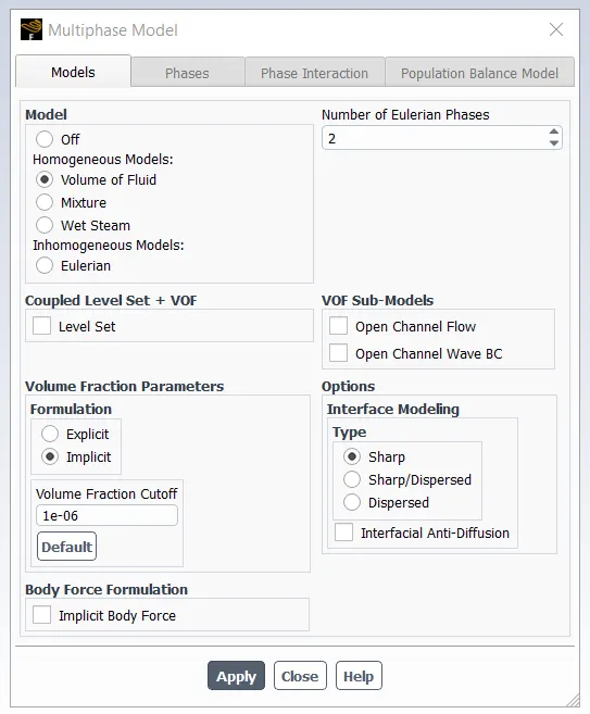
We enable the multiphase model (Volume of Fluid homogeneous model) with 2 Eulerian phases, as we are dealing with two phases, being air and the lubricant fluid. We use the implicit formulation, as the explicit method tends to increase the Courant number substantially, during the simulation.

Material Selection :

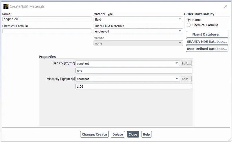
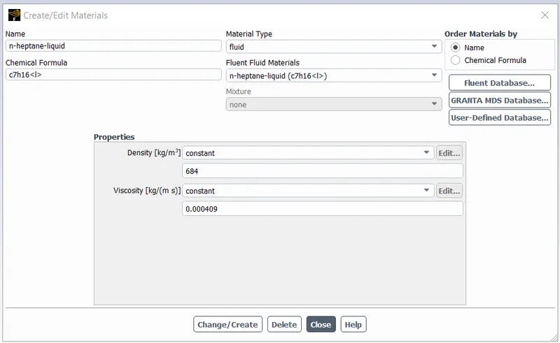
In this step, we select the lubricant materials which are circulated around the gears, along with air. The lubricants used for this simulation are as follows.

1. Engine Oil

Engine oil must lubricate the various parts of an engine to reduce friction and minimize unnecessary loss of power. A well lubricated engine will burn fuel more effectively and therefore perform better.

2. n – heptane (C7H16)

n-heptane is defined as the zero point of the octane rating scale. It is a lighter component in gasoline, burns more explosively, causing engine pre-ignition (knocking) in its pure form.

User – Defined Function (UDF) :

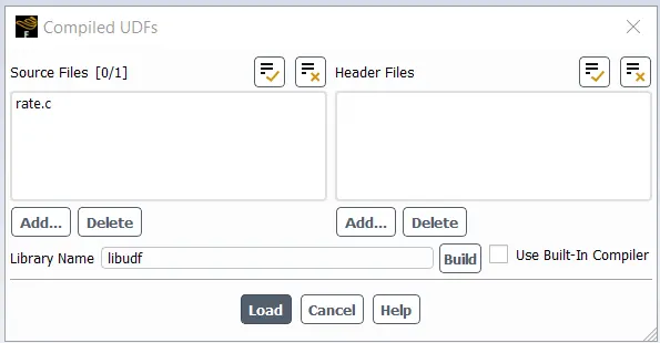
In this step, the user – defined function file containing the information describing the moving zones of the left and right gears is loaded into fluent. We use the compiled user – defined function option to build and load the source file.

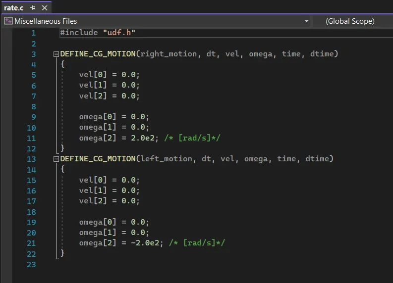
The user – defined function is given by,

After successfully loading the UDF into fluent, we then move on to create a dynamic meshing for the geometry.

Dynamic Meshing :

Dynamic meshing is used to model flows where the shape of the domain is changing with time due to motion on the domain boundaries. Generally, the dynamic mesh technique simulates models that require a moving mesh area.

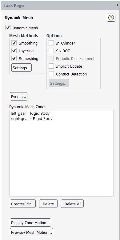
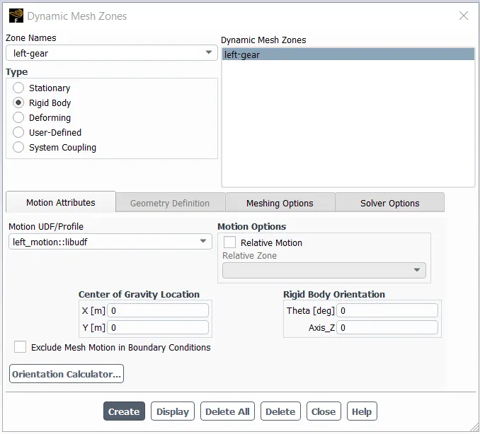
Further, we create two individual profiles representing the motion of the left and right gears. As the centre of gravity of the left gear is at the origin, we represent it as follows.

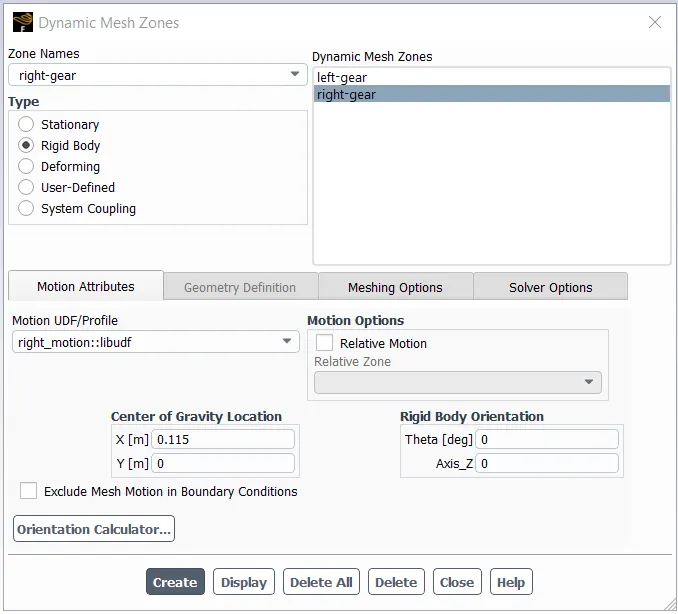
As the centroid of centre of gravity of the right gear is at a distance of 115 mm (0.115 m) from the origin, we represent its properties as follows.

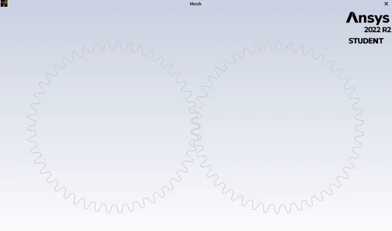
Thereby creating the two dynamic meshing zones, we then display the zone motion so as to visualize the movement of the gears, with respect to each other.

Marking Cells :

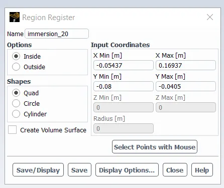
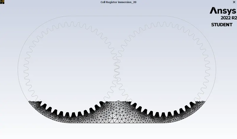
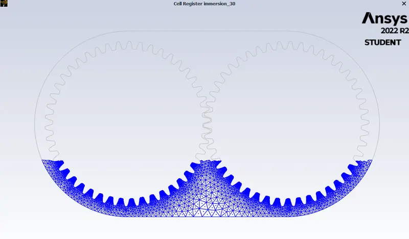
In this step, we define new cell registers, defining the regions which represent the levels of immersion of the fluid. We do this by creating a new region with reference to the co-ordinates of the bounding box as previously calculated.

The marked cells of different immersion level are as follows.

20% immersion level :

The dimensions of the region to be marked.

The region of marked cells is shown by.

30% immersion level :

The dimensions of the region to be marked.

Marked region.

CASE – 1 : 20% immersion, Fluid – Engine Oil

To carry out the simulation, we first setup the general case parameters as shown above. Next, we modify the phases with accordance to the lubricant material we are going to use.

In this case, as we are using engine oil, the secondary phase material will be considered as engine – oil. The primary phase material with which the engine oil mixes with is considered to be air.

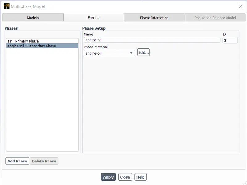
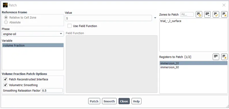
We then hybrid initialize the setup. Further, we use the patch command to patch the value of engine oil onto the marked cells of 20% immersion. We provide the value of volume fraction as 1 for engine oil.

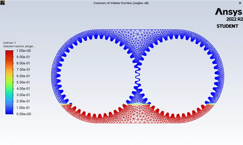
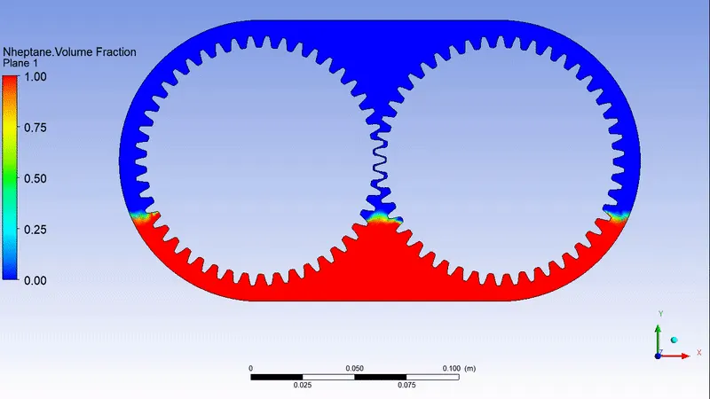
To visualize the patch, we create a phase contour representing the volume fractions of the different materials. The fluid interaction region along with the immersed fluid level is visualized as shown. The blue region represents air inside the housing and the red region represents the lubricant.

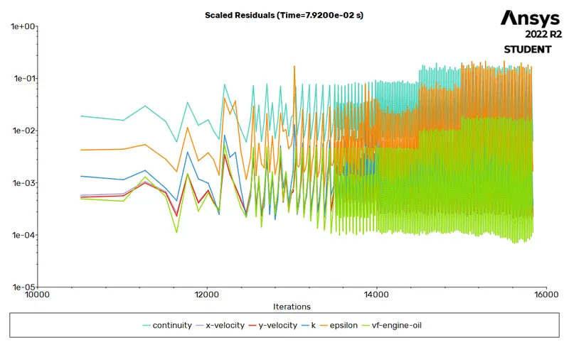
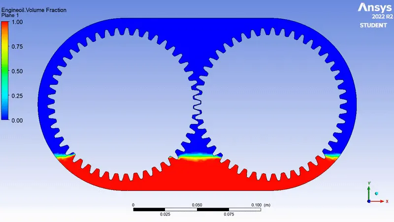
Finally, we run the simulation for a time-step size of 0.0001 and for 600 time-steps. We also create a solution animation so as to visualize the results at each and every timestep. The following results are obtained from the simulation.

Residuals Plot :

Solution Animation :

CASE – 2 : 30% immersion, Fluid – Engine Oil

After setting up the general case parameters, we then mark the cells upto the 30% immersion level mark, with respect to the co-ordinates previously calculated. We then patch the volume fraction value of engine to the 30% immersion region by representing its value as 1.

The initial volume fraction contour is as represented below.

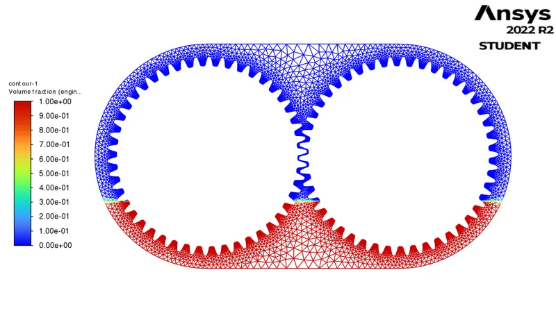
By running the simulation at a timestep size of 0.0001 for 600 time-steps, we obtain the following results.

Residuals :

Solution Animation :

CASE – 3 : 20% immersion, Fluid :– n-heptane (C7H16)

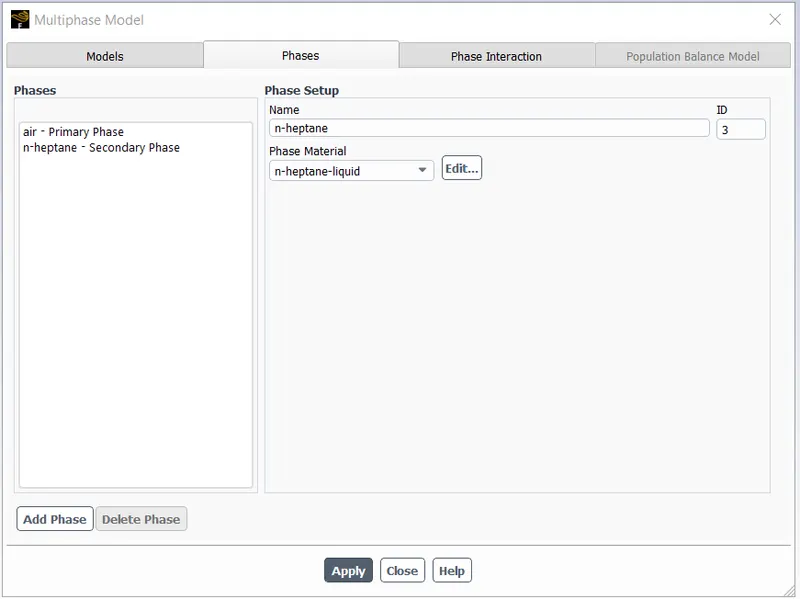
For this simulation, we consider the primary phase to be air and the secondary phase, i.e., the lubricant as n – heptane (C7H16). Thereby, we add this in the materials library and assign it to the secondary phase material.

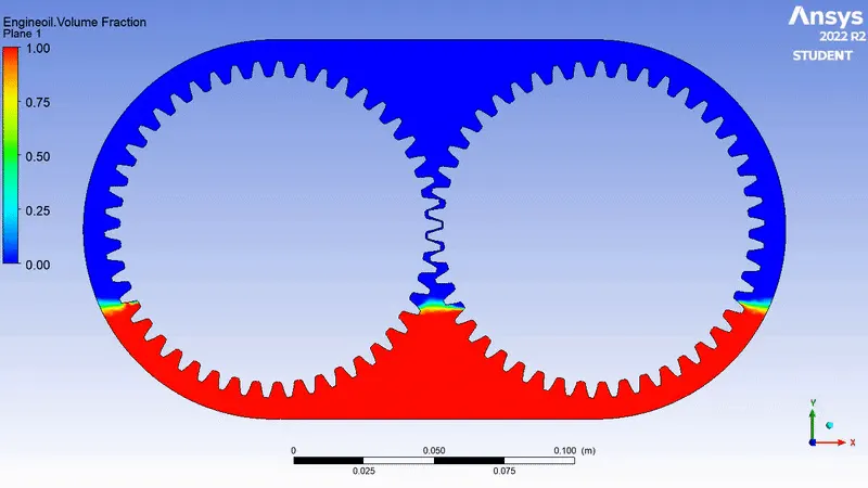
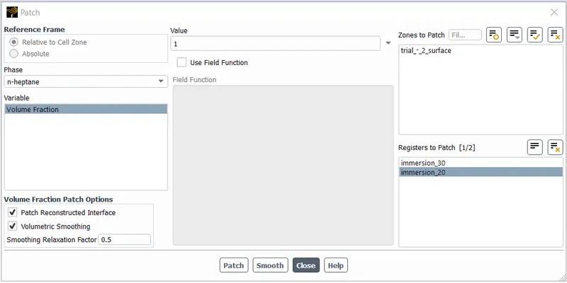
Further, we hybrid initialize the simulation and patch the volume fraction value of n-heptane as 1, representing the 20% immersion region.

We thereby obtain the volume fraction contour as follows.

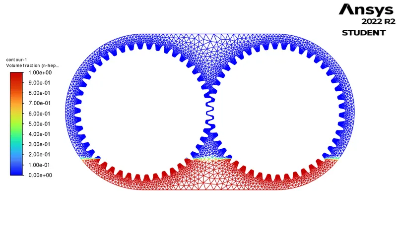
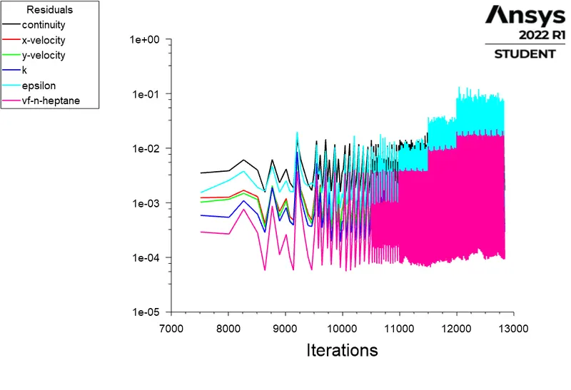
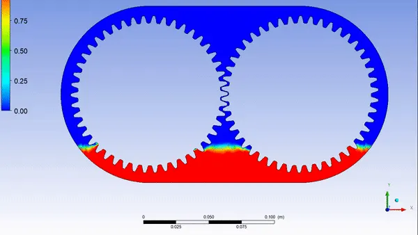
Running the simulation for a timestep size of 0.0001 and for 600 time-steps, we obtain the following results.

Residuals Plot :

Solution Animation :

CASE – 4 : 30% immersion, Fluid :– n-heptane (C7H16)

For this case study, for the same lubricating fluid (n-heptane), we consider the 30% immersion level of the fluid. Thereby, we hybrid initialize the simulation and patch the volume fraction value of n-heptane as 1, representing the 30% immersion region.

The volume fraction contour is represented by,

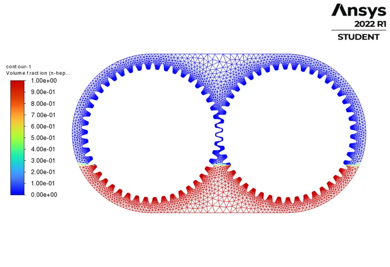
Running the simulation for a timestep size of 0.0001 and for 700 time-steps, we obtain the following results.

Residuals Plot :

Solution Animation :

Calculation of Rotational Parameters :

From the UDF file, we have the value of the rotational speed of the gears as 200 radians / second.

As we know, the formula for angular velocity is given by,

`omega = (2piN)/60`

Where,

`omega` = Angular Velocity (rad/sec) = 200 rad/sec

`N` = Number of Rotations per minute (rpm)

Therefore, the rotational speed is calculated as,

`200=(2⋅π⋅N)/60`

`N=6000/π`

N = 1909.85 rpm

Calculating the number of rotations per second (rps), we get

`N=1909.85/60`

N = 31.83 rps

Therefore, the time taken for one rotation is calculated as,

`"Time" =1/31.83`

Time = 0.03141 seconds.

Hence, the time required to complete one rotation of the gear is 0.03141 seconds.

PART – 2 : THEORETICAL DISCUSSIONS

In this section, we are going to talk about the various theoretical aspects related to the simulation.

What is dynamic meshing? Give some examples where dynamic meshing can be used.

The dynamic mesh model can model flows where the domain’s shape changes with time due to motion on the domain boundaries. Combined with the six degrees of freedom (6 DOF) solver, dynamic mesh allows the trajectory of a moving object to be determined by the aero or hydrodynamic forces from the surrounding flow field. In ANSYS Fluent, the dynamic mesh capability is used to simulate problems with boundary motion, such as check valves and store separations. Generally, the dynamic mesh technique simulates models that require a moving mesh area.

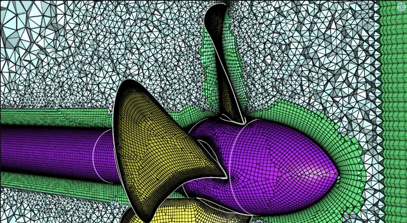
The building blocks for dynamic mesh capabilities within ANSYS FLUENT are three dynamic mesh schemes: smoothing, layering and remeshing. Combining these three schemes is used to tackle the most challenging dynamic mesh problems.

1. Smoothing Method

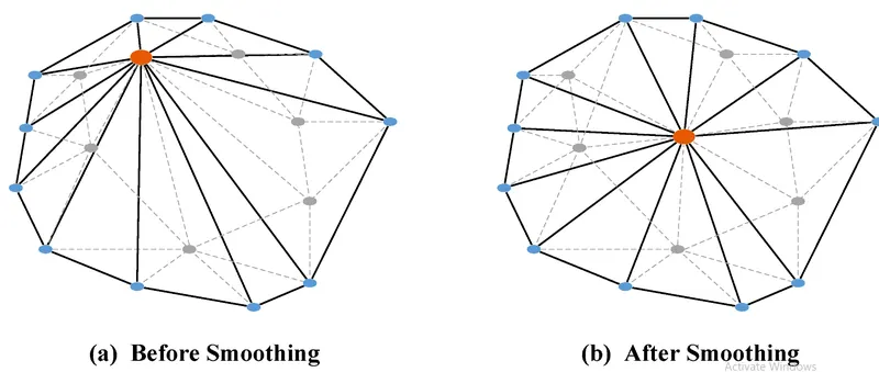
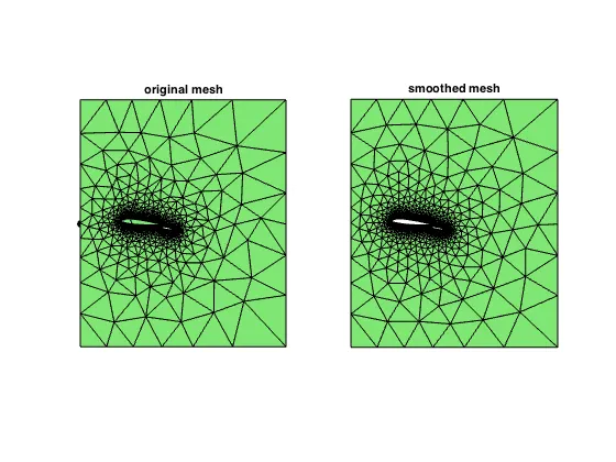
The smoothing method adjusts the mesh of an area by moving or deforming boundaries, but the number of nodes and connections does not change.

2. Layering Method

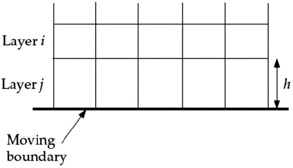
The dynamic layering method is used when multilayers of cells are added to or subtracted from the cell layer adjacent to the moving boundary. This can be based on the layer height.

3. Remeshing Method

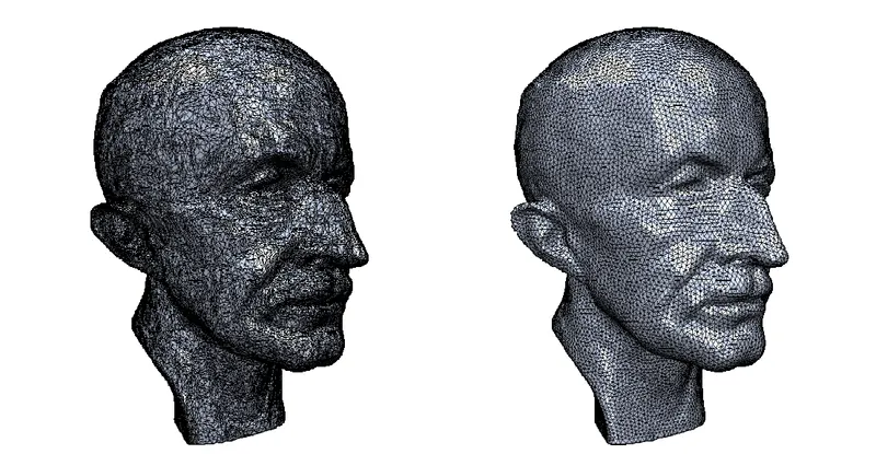
The remeshing method is used for situations where the boundary displacement is large compared to the size of the local cells, which causes the cell quality to deteriorate; thus, the mesh becomes invalid. For example, a negative cell volume error may occur, eventually leading to a problem-solving divergence at the next step. Therefore, it compresses cells that disrupt the skewness value or critical size limit and locally remeshes the meshed cells or surfaces to address this problem. If the new cells satisfy the critical skewness value, the mesh is updated locally with the new cells; otherwise, the new cells are discarded, and the same old cells remain.

Some of the few instances where dynamic meshing can be used in real life are as follows,

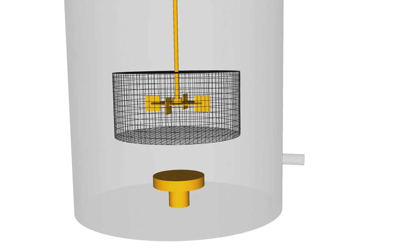
1. Sliding meshes in stirrer tanks.

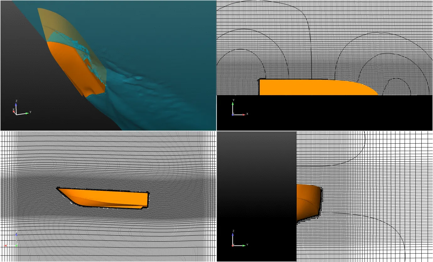
2. Mesh morphing and rigid body motion of a boat moving on water.

3. Mesh deformations around a fish swimming in water.

4. Oversetting mesh of an overtaking car.

What is the fluid Sloshing effect? Discuss whether the sloshing effect is good or bad?

Sloshing means any motion of the free liquid surface inside its container. It is caused by any disturbance to partially filled liquid containers. Such motion is characterized by "inertial waves".

The basic problem of liquid sloshing involves the estimation of hydrodynamic pressure distribution, forces, moments and natural frequencies of the free-liquid surface. These parameters have a direct effect on the dynamic stability and performance of moving containers.

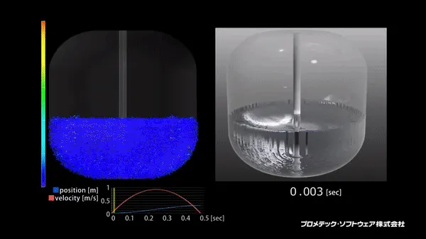
Important examples include propellant slosh in spacecraft tanks and rockets (especially upper stages), and the free surface effect (cargo slosh) in ships and trucks transporting liquids (for example oil and gasoline), water sloshing in the swimming pool of a cruise ship etc.

What is the use of UDF?

A UDF is basically a C program or a C function that can be dynamically loaded with ANSYS FLUENT to enhance its standard features. For example, you can use a UDF to define your own boundary conditions, material properties, and source terms for your flow regime, as well as specify customized model parameters (e.g., DPM, multiphase models), initialize a solution, or enhance post-processing.

UDFs are written in the C programming language using any text editor and are coded using additional macros and functions. The source code file is saved with a “.c” extension (e.g., myudf.c). One source file can contain a single UDF or multiple UDF’s.

Source files containing UDFs can be either interpreted or compiled in ANSYS FLUENT. For interpreted UDFs, source files are interpreted and loaded directly at runtime, in a single-step process. For compiled UDFs, the process involves two separate steps. A shared object code library is first built and then it is loaded into ANSYS FLUENT. After being interpreted or compiled, UDFs will become visible and selectable in ANSYS FLUENT dialog boxes, and can be hooked to a solver by choosing the function name in the appropriate dialog box.

Discuss the common errors that occurred in the simulation.

A] 'Dynamic mesh failed' error.

Most times, these types of problem come as a result of bad mesh quality. Both for the unstructured and structured mesh, do a quick mesh quality check and remesh if found to be poor.

Check the size of the smallest volume. It can happen that also a very small motion of the boundaries implies the collapse of one element. Furthermore, check the diffusivity of the mesh motion.

B] 'Negative cell volume detected' error.

The negative cell volume error is shown when the mesh has been updated in a way to cause a negative cell volume (non-physical). Possible factors for causing this error include:

1.) Overlapping nodes.

2.) Significant mesh motion (relative to cell size) per step.

These factors are related and you could try to reduce the time step to avoid major mesh displacements.