Week 2 - Flow over a Cylinder.
AIM :
To simulate the flow over a cylinder and explain the phenomenon of Karman vortex street.
OBJECTIVES :
- To simulate the flow over a cylinder, for the steady and unsteady case and calculate the Strouhal Number for Re= 100.
- Calculate the coefficient of drag and lift over a cylinder by setting the Reynolds number to 10, 100, 1000, 10000 & 100000, by using the steady solver.
- Discuss the effect of Reynolds number on the coefficient of drag and validate the results (error should be within 5 %).
INTRODUCTION :
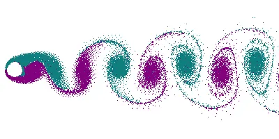
Flow past a blunt body, such as a circular cylinder, usually experiences boundary layer separation and very strong flow oscillations in the wake region behind the body. In certain Reynolds number range, a periodic flow motion will develop in the wake as a result of boundary layer vortice being shed alternatively from either side of the cylinder. This regular pattern of vortices in the wake is called a Karman vortex street. It creates an oscillating flow at a discrete frequency that is correlated to the Reynolds number of the flow.
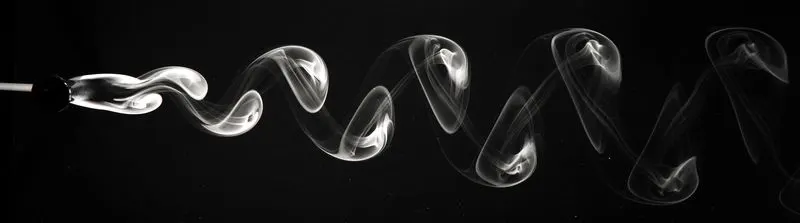
Visualisation of the Karman vortex street in the wake behind a circular cylinder in air
The characteristics of flow separation at different Reynold’s Numbers are as shown below,
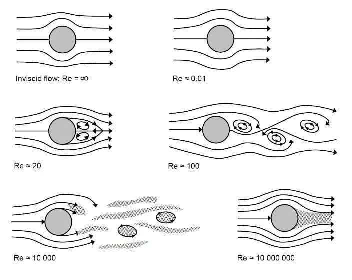
Flow over a cylinder is important in many industrial applications like cooling of iron or cylindrical pipe. Circular pipes have more application in heat exchanger, where high temperature flue gases flow over a circular cylinder in a cross flow.
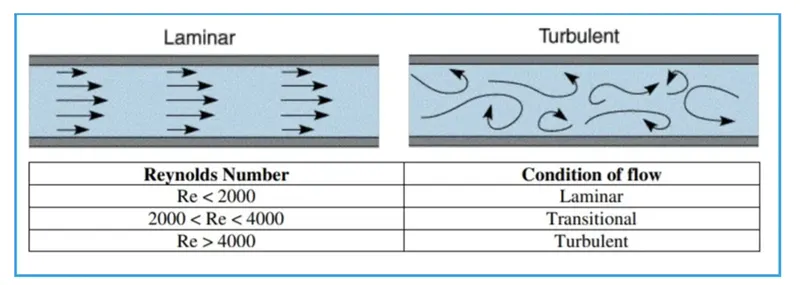
Depending on flow rate, fluid properties and size of cylinder, the flow can be laminar, transitional and turbulent.
Wake :
Wake is the region of recirculating flow immediately behind a moving or stationary blunt body, caused by viscosity, which may be accompanied by flow separation and turbulence. It is basically the region of disturbed flow downstream of a solid body moving through a fluid.
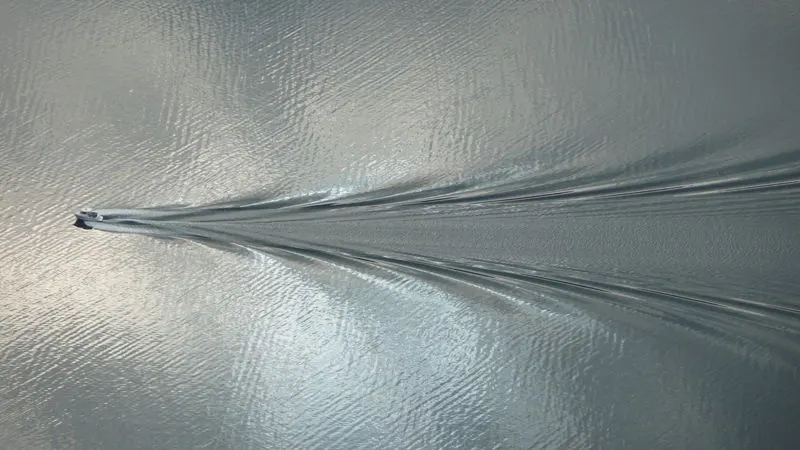
Wake pattern created by a small boat
Reynold’s Number :
Reynold’s number is a dimensionless quantity that is used to determine the type of flow pattern as laminar or turbulent while flowing through a pipe. Reynolds number is defined by the ratio of inertial forces to that of viscous forces.
`"Reynold’s number" = "Inertial Force" / "Viscous Force"`
The formula is given by,
`R_e = (v*D)/nu`
Where,
`D` = Diameter of Cylinder (`m`)
`v` = Velocity of Fluid (`m` /`s`)
`nu` = Kinematic Viscosity of Fluid (`m^2`/`s`).
Strouhal Number :
Strouhal number is a dimensionless number describing oscillating flow mechanisms. The Strouhal Number represents a measure of the ratio of the inertial forces due to the unsteadiness of the flow or local acceleration to the inertial forces due to changes in velocity from one point to another, in the flow field.
The frequency at which vortex shedding takes place for an infinite cylinder is related to the Strouhal number.
The Strouhal number is often given as,
`St = (f*L)/U`
Where,
`f` = Frequency of Vortex Shedding
`L` = Characteristic Length (for example, hydraulic diameter or the airfoil thickness)
`U` = Flow Velocity.
Vortex Shedding :
Vortex shedding is an oscillating flow that takes place when a fluid such as air or water flows past a bluff (as opposed to streamlined) body at certain velocities. In this flow, low-pressure vortices are created at the back of the body (downstream side) and detach periodically from either side of the body forming a Von Kármán vortex street. The object will tend to move toward the low-pressure zone.
The vortex shedding occurs at a discrete frequency and is a function of the Reynolds number.
Lift Co-efficient :
The lift coefficient (`C_L`) is a dimensionless coefficient that relates the lift generated by a lifting body to the fluid density around the body, the fluid velocity and an associated reference area. `C_L` is a function of the angle of the body to the flow, its Reynolds number and its Mach number.
`C_L = F_L / (1/2 * rho * A * v^2)`
Where,
`F_L` = Lift Force
`rho` = Fluid Density
`A` = Projected Area of Object with respect to which lift force is calculated
`v` = Flow Velocity.
Drag Co-efficient :
Drag coefficient is a dimensionless quantity that is used to quantify the drag or resistance of an object in a fluid environment, such as air or water. A lower drag coefficient indicates the object will have less aerodynamic or hydrodynamic drag. The drag coefficient is always associated with a particular surface area.
`C_D = F_D / (1/2 * rho * A * v^2)`
Where,
`F_D` = Drag Force
`rho` = Fluid Density
`A` = Projected Area of Object with respect to which drag force is calculated
`v` = Flow Velocity.
COMPUTATIONAL DOMAIN :
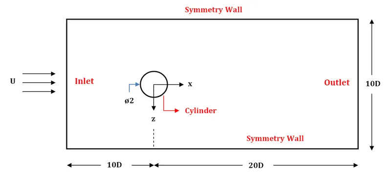
The computational domain for the flow over a cylinder is given by,
SIMULATION PROCEDURE :
With reference to the above shown domain, we are going to carry out our simulation using the ANSYS Workbench software by the following steps.
1. GEOMETRY
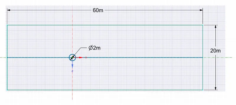
In this step, we are going to design our geometry using the above mentioned specifications. We obtain a 2-D model as shown below.
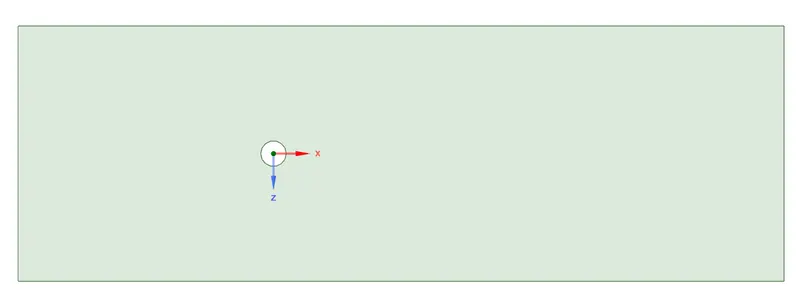
We use the “pull” option to form the hole in the geometry and thereby obtaining the final model as shown below.
2. MESHING
In this step, we are going to generate meshing for the obtained geometry.
- First, we are going to insert a method to change the quadrilateral dominated meshing to a triangular meshing.
- We create the meshing for an element size of 0.25 m, to obtain a fine mesh so as to precisely capture the details of the simulation.
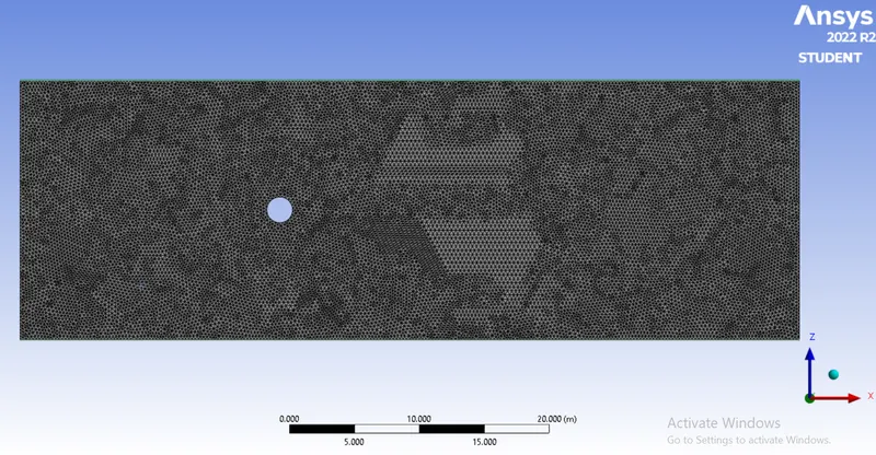
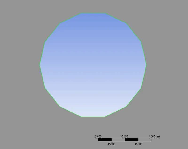
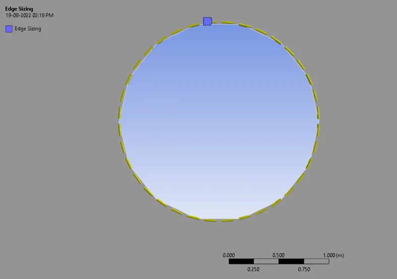
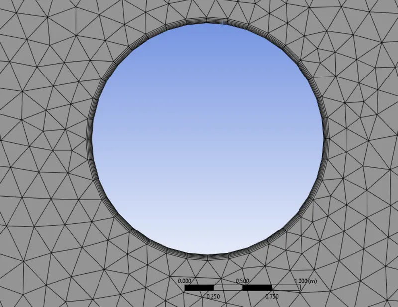
Zooming into the circle, we can observe that it is more of a polygon with 14 sides. These sharp edges or sides impact the flow field around the circle. So to prevent this, we further refine the circle by using the edge sizing option in which we create a circle with 36 divisions (1 division per every `10^o`) and thereby obtaining a smoother circle.
Before After
Final Result :
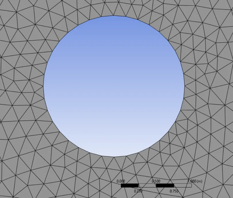
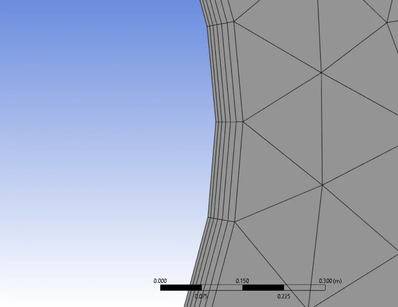
Since the fluid flow around the cylinder is our main study of interest, we need to precisely capture the details pertaining to that. To do so, we create an inflation layer, which helps us create a body fitted mesh.
We create 6 layers of 5 mm thickness, with a growth rate of 1.2 (20%), as shown.
The last step of the meshing process is creating the named selections of the faces to define the inlet, outlet, wall and the symmetry conditions of the geometry.
3. SETUP & SOLUTION
The first and foremost step in simulation setup is to make sure all the components of the geometry have been imported into the ANSYS Fluent software and to also perform a mesh check.
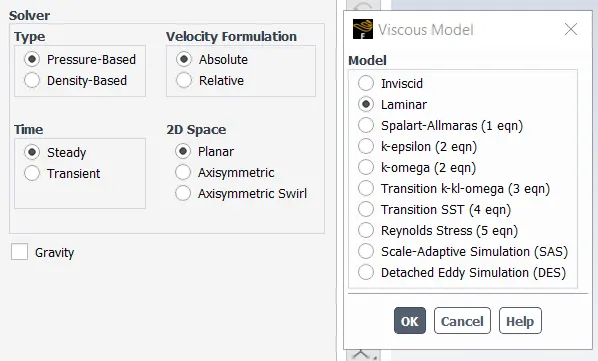
We choose a steady state pressure – based solver with absolute velocity formulation, to run the simulation. Also, we select a laminar viscous model to simulate streamline fluid flow.
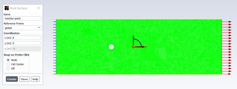
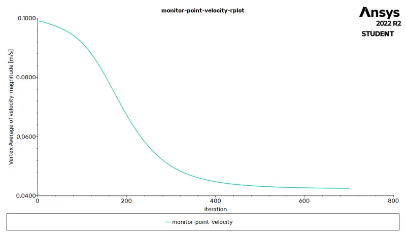
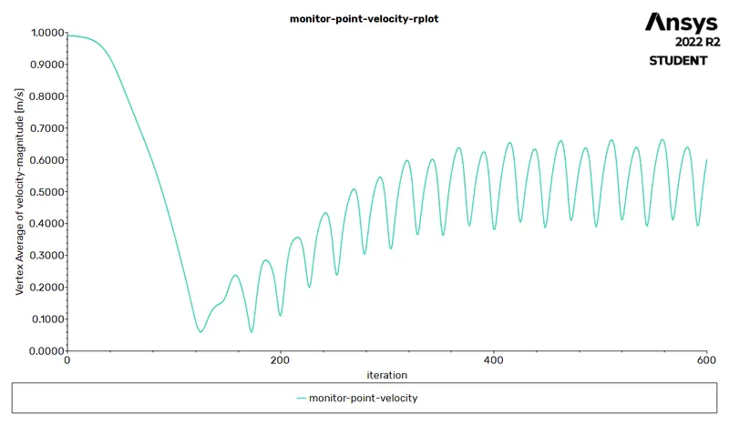
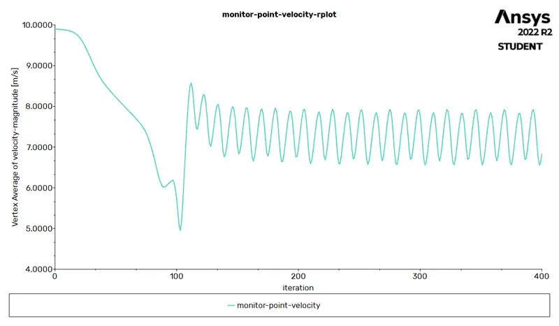
In the next step, we create a monitor point to observe the characteristics of flow at a certain point in the domain (in the Karman Vortex Street). This monitor point is at a distance of 4D from the centre of the circle.
In the next step, we setup 5 cases to simulate the fluid flow at different Reynold’s Numbers. We modify the Reynold’s Number by varying the inlet velocity of the flow.
CASE – 1 : REYNOLD’S NUMBER (Re) = 10
Reynold’s Number `R_e = 10`
Fluid Inlet Velocity `v = 0.1` `m`/`s`
Density of Material `rho = 1` `kg`/`m^3`
Viscosity `nu = 0.02` `kg`/`m*s`
By running the simulation for the above mentioned specifications, we get the output results as follows.
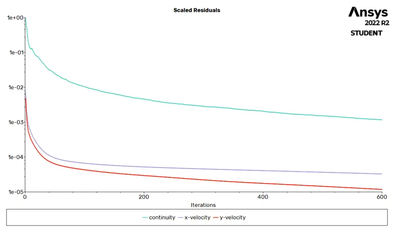
Residual Plot :
Monitor Point Velocity :
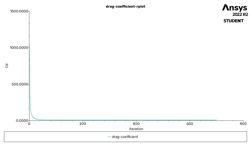
Drag Co-efficient :
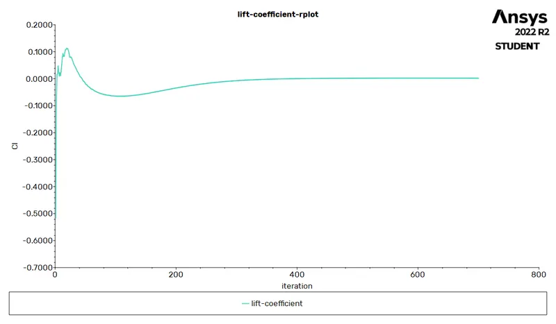
Lift Co-efficient :
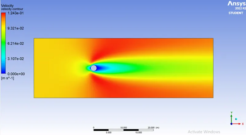
Velocity Contour Plot :
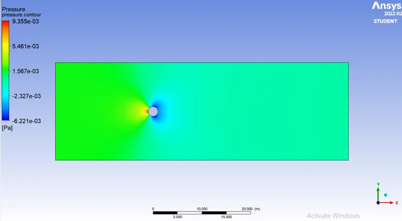
Pressure Contour Plot :
Output Parameters :
Drag Co-efficient = 5.4348
Lift Co-efficient = 0.0011
CASE – 2 : REYNOLD’S NUMBER (Re) = 100
Reynold’s Number `R_e = 100`
Fluid Inlet Velocity `v = 1` `m`/`s`
Density of Material `rho = 1` `kg`/`m^3`
Viscosity `nu = 0.02` `kg`/`m*s`
For this case, we are going to have two sub-cases for which we are going to run the simulation for both the steady state and unsteady state methods and compare the difference.
Case 2.1 : Steady State
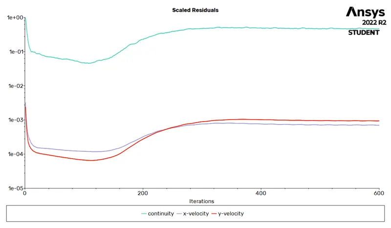
In this sub-case, we are going to run the simulation for 600 iterations, at a steady time state.
Residual Plot :
Monitor Point Velocity :
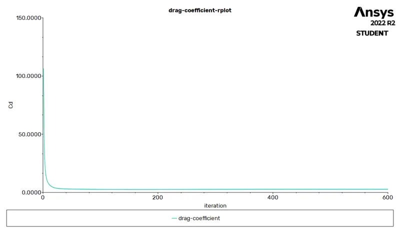
Drag Co-efficient :
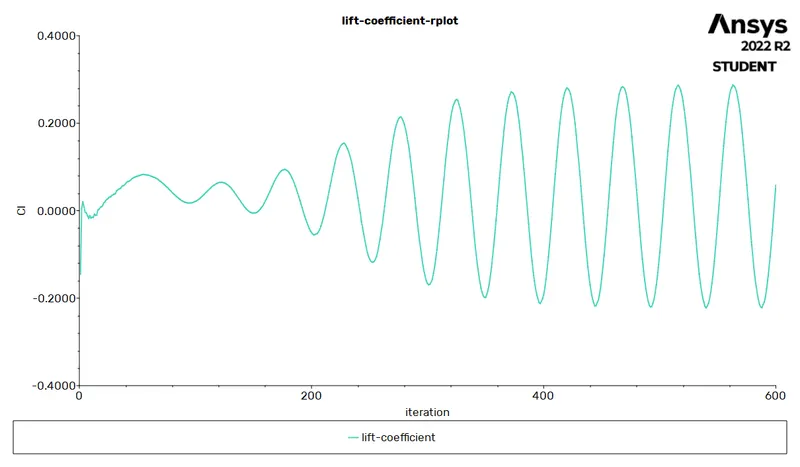
Lift Co-efficient :
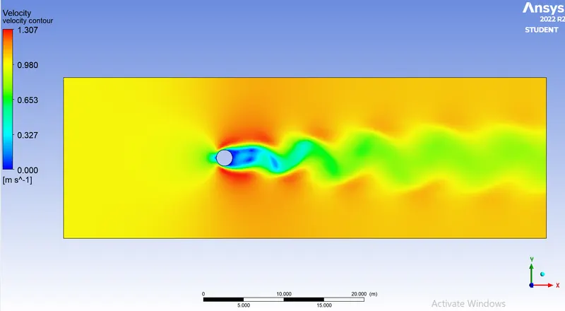
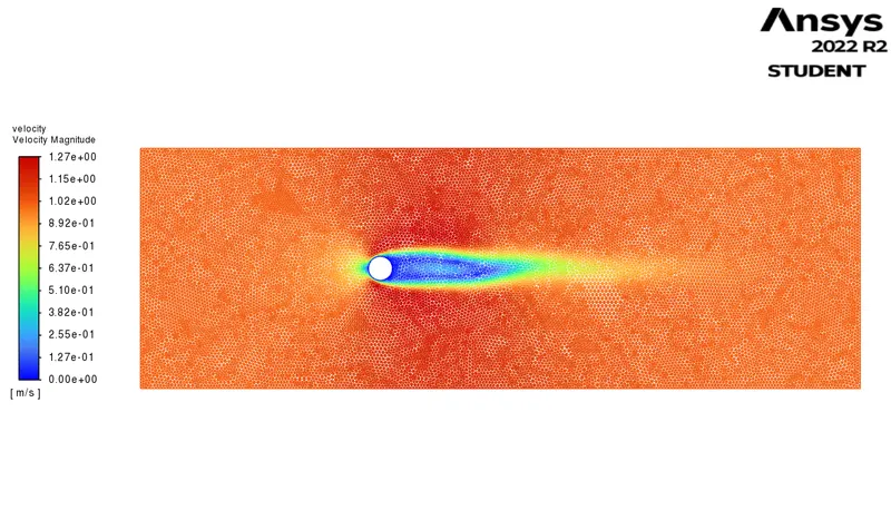
Velocity Contour Plot :
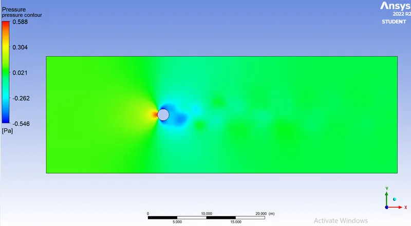
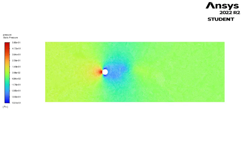
Pressure Contour Plot :
Output Parameters :
Drag Co-efficient = 1.3043
Lift Co-efficient = 0.0319
Case 2.2 : Unsteady State
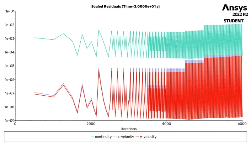
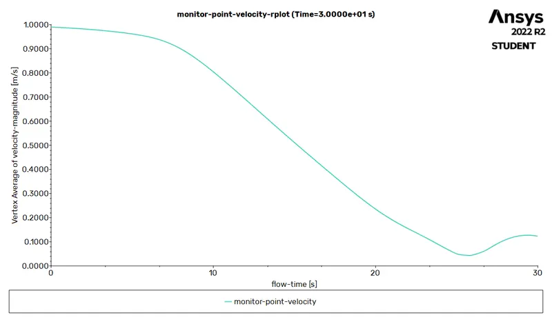
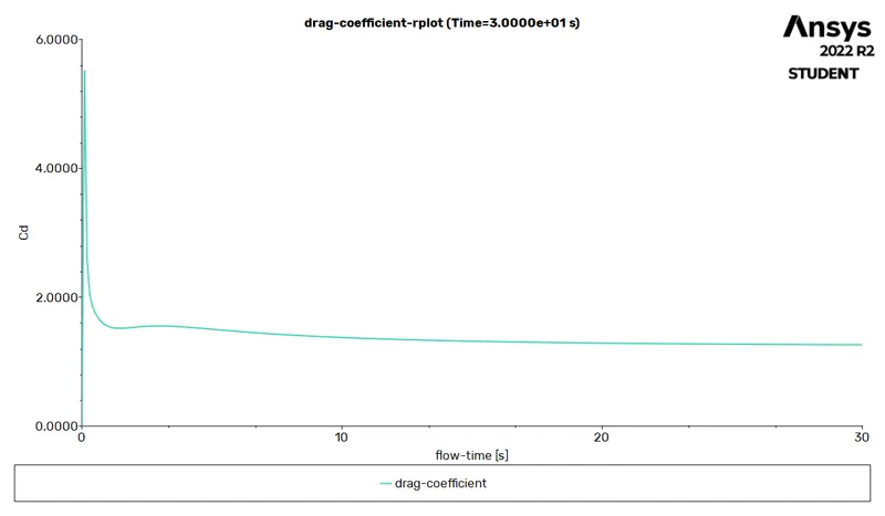
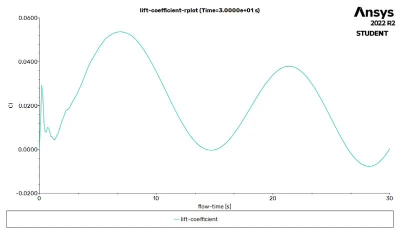
In this sub-case, we are going to run the simulation for 300 time-steps, at an unsteady time state.
Residual Plot :
Monitor Point Velocity :
Drag Co-efficient :
Lift Co-efficient :
Velocity Contour Plot :
Pressure Contour Plot :
Output Parameters :
Drag Co-efficient = 1.2826
Lift Co-efficient = 0.0305
CASE – 3 : REYNOLD’S NUMBER (Re) = 1000
Reynold’s Number `R_e = 1000`
Fluid Inlet Velocity `v = 10` `m`/`s`
Density of Material `rho = 1` `kg`/`m^3`
Viscosity `nu = 0.02` `kg`/`m*s`
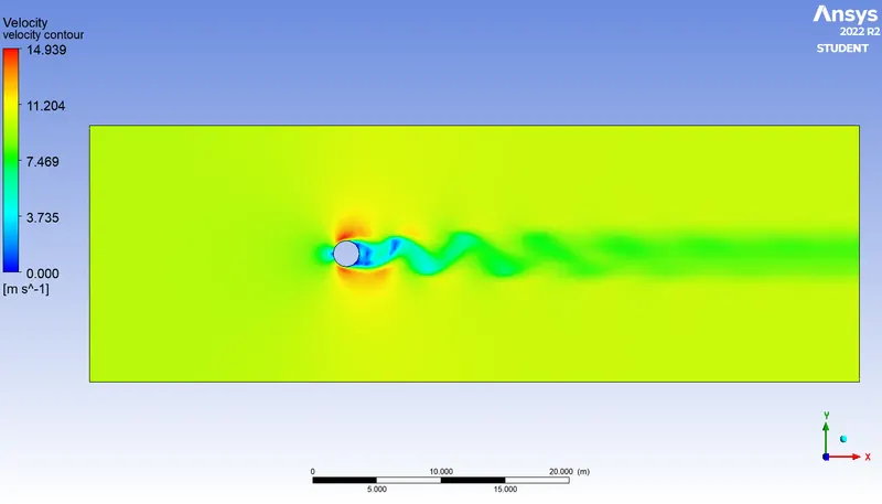
In this case setup, we are going to increase the inlet velocity of the fluid flow to bring up the Reynold’s Number to 1000 and study the characteristics.
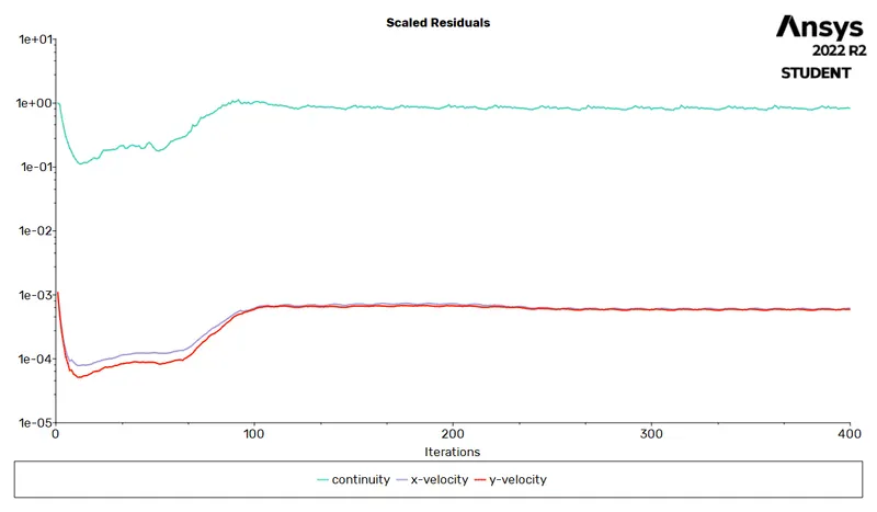
Residual Plot :
Monitor Point Velocity :
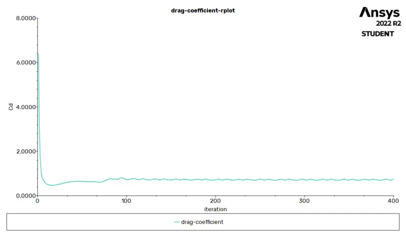
Drag Co-efficient :
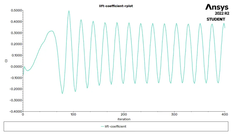
Lift Co-efficient :
Velocity Contour Plot :
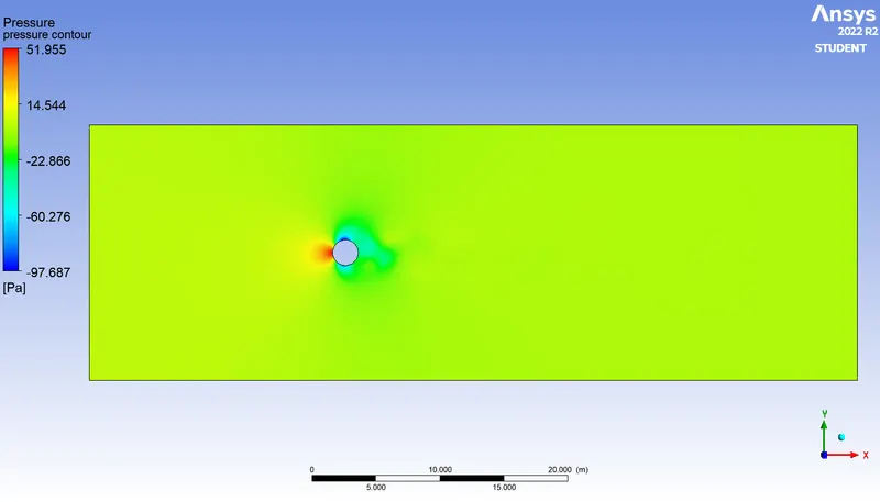
Pressure Contour Plot :
Output Parameters :
Drag Co-efficient = 0.7681
Lift Co-efficient = 0.2304
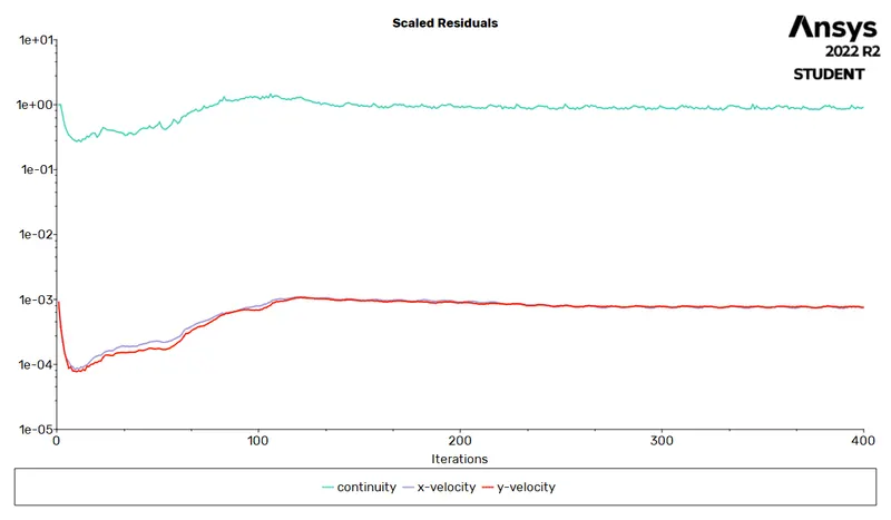
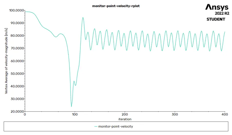
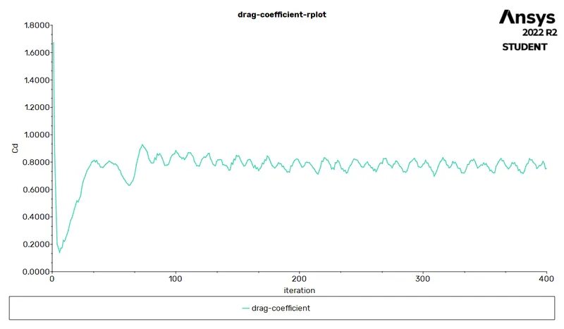
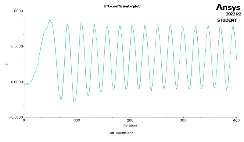
CASE – 4 : REYNOLD’S NUMBER (Re) = 10000
Reynold’s Number `R_e = 10000`
Fluid Inlet Velocity `v = 100` `m`/`s`
Density of Material `rho = 1` `kg`/`m^3`
Viscosity `nu = 0.02` `kg`/`m*s`
Residual Plot :
Monitor Point Velocity :
Drag Co-efficient :
Lift Co-efficient :
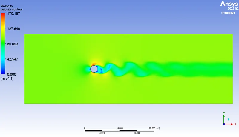
Velocity Contour Plot :
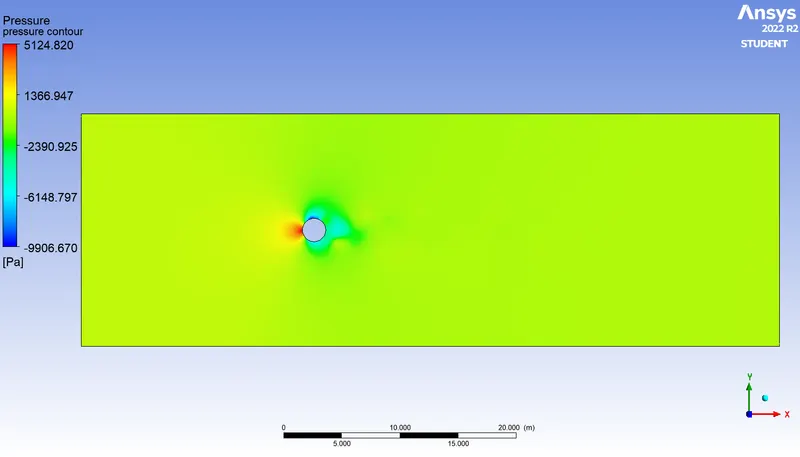
Pressure Contour Plot :
Output Parameters :
Drag Co-efficient = 0.7565
Lift Co-efficient = 0.7038
CASE – 5 : REYNOLD’S NUMBER (Re) = 100000
Reynold’s Number `R_e = 100000`
Fluid Inlet Velocity `v = 1000` `m`/`s`
Density of Material `rho = 1` `kg`/`m^3`
Viscosity `nu = 0.02` `kg`/`m*s`
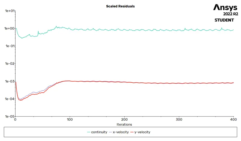
Residual Plot :
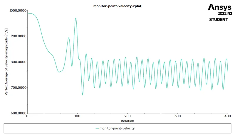
Monitor Point Velocity :
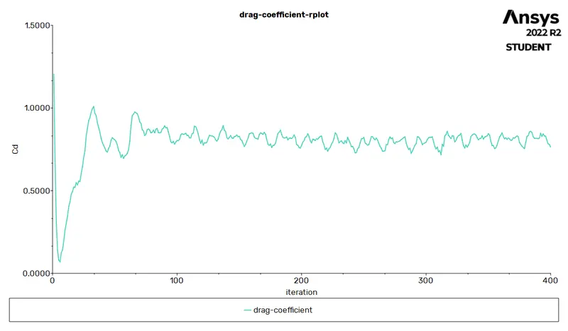
Drag Co-efficient :
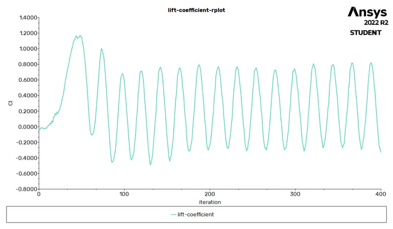
Lift Co-efficient :
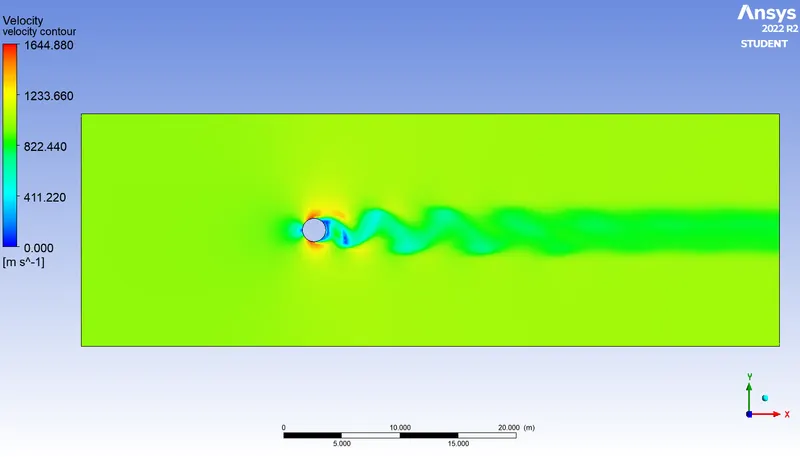
Velocity Contour Plot :
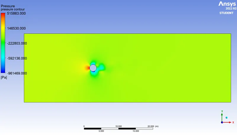
Pressure Contour Plot :
Output Parameters :
Drag Co-efficient = 0.7192
Lift Co-efficient = 0.4525
VALIDATION :
To validate our results, we calculate the Strouhal Number for Reynold’s Number, Re = 100 and then we compare it with the graphical value obtained (numerical value).
As we know,
`St = (f*L)/U`
Where,
`f` = Frequency of Vortex Shedding = 0.0312
`L` = Characteristic Length (diameter in this case) = 2 m
`U` = Flow Velocity = 1 m/s
`therefore` `St = (0.0312 xx 2)/1` = 0.0624 `->` Analytical Value
Numerical Value :
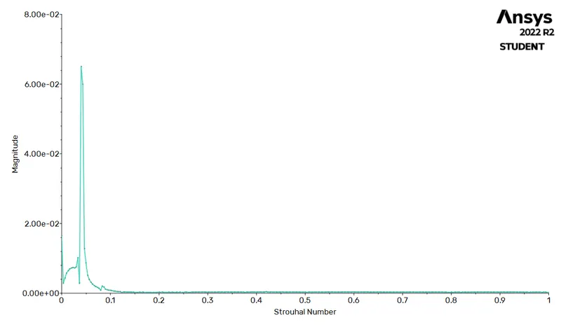
Strouhal Number (Numerical) = 0.06312

Thereby, the analytical results have been validated with the numerical solution with an error percentage of less than 5%.
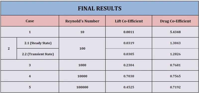
FINAL RESULTS :
The final results of all the 5 case studies have been tabulated as follows.
CONCLUSION :
The fluid flow over a cylinder has successfully been simulated for the Reynold’s Numbers – 10 , 100 , 1000 , 10000 and 100000 and the respective plots and contours have been obtained.
From the plots and contours, we can observe that no significant vortex shedding is observed in very low Reynold’s Numbers. Therefore, to observe the vortex shedding phenomenon, we need to simulate the flow at higher Reynold’s numbers by increasing the fluid velocity at the inlet.
Also, from the simulations run, we can observe that the transient state simulation takes a very high simulation time to compute the results and the number of iterations or timesteps it takes to reach a steady state is also very high. Therefore, transient state simulation requires much higher simulation time and the time taken to reach a steady state is very high.
From the numerical results obtained from the simulation, we can observe that as the Reynold’s Number increases, the drag co-efficient is substantially decreasing. This means that, at high Reynold’s numbers, the effect of drag due to the boundary layer is less.