Week 8 - Simulating Cyclone separator with Discrete Phase Modelling
AIM :
To perform analysis on cyclone separator and calculate the separation efficiency and pressure drop.
OBJECTIVES :
- Describe any four empirical models used to calculate the cyclone separator efficiency.
- Perform an analysis on the given cyclone separator model by varying the particle diameter from 1 μm to 5 μm and calculate the separation efficiency in each case. Discuss the results. [Use both the velocities as 3 m/sec].
- Perform an analysis on the given cyclone separator model by varying the particle velocity from 1m/sec to 5 m/sec and calculate the separation efficiency and pressure drop in each case. Discuss the results. [Use particle diameter size as 5 μm for all cases & keep flow velocity same as particle velocity].
INTRODUCTION :
Cyclone separators or simply cyclones are separation devices that use the principle of inertia to remove particulate matter from flue gases. Cyclone separators are one of many air pollution control devices known as precleaners since they generally remove larger pieces of particulate matter. This prevents finer filtration methods from having to deal with large, more abrasive particles later on.
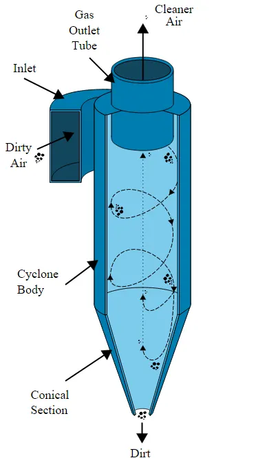
Most cyclones are built to control and remove particulate matter that is larger than 10 micrometers in diameter. However, there do exist high efficiency cyclones that are designed to be effective on particles as small as 2.5 micrometers. As well, these separators are not effective on extremely large particulate matter. For particulates around 200 micrometers in size, gravity settling chambers or momentum separators are a better option.
How It Works :
Cyclone separators work much like a centrifuge, but with a continuous feed of dirty air. In a cyclone separator, dirty flue gas is fed into a chamber. The inside of the chamber creates a spiral vortex, similar to a tornado. The lighter components of this gas have less inertia, so it is easier for them to be influenced by the vortex and travel up. Contrarily, larger components of particulate matter have more inertia and are not as easily influenced by the vortex.
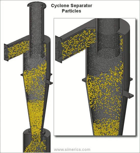
Since these larger particles have difficulty following the high-speed spiral motion of the gas and the vortex, the particles hit the inside walls of the container and drop down into a collection hopper. These chambers are shaped like an upside-down cone to promote the collection of these particles at the bottom of the container. The cleaned flue gas escapes out the top of the chamber.
Efficiency of Cyclone Separator :
The collection efficiency, also known as the capture or recovery rate - is a measurement of a cyclone’s ability to separate particles from the flowing gas stream. Because particles have different sizes, the efficiency rating is usually given for varying particle sizes.
In this simulation, the separation efficiency of the cyclone separator is calculated as,
`"Separator Efficiency" = "Trapped Particles" / "Tracked Particles" xx 100`
There are several factors that can affect a cyclone separators efficiency. These include particle density, particle size, volumetric flow rate, pressure drop, cone length, body length, ratio of accept port to body diameter, and even the smoothness of the cyclone’s internal surfaces.
A few of the empirical models used to calculate the cyclone separator efficiency are as follows.
1. IOZIA AND LEITH MODEL
Iozia and Leith logistic model is developed based on force balance. The model assumes that a particle carried by the vortex endures the influence of two forces : a centrifugal force “Z”, and a flow resistance “W”.
The collection efficiency `eta_i` of particle diameter `d_"pi"` can be calculated from,
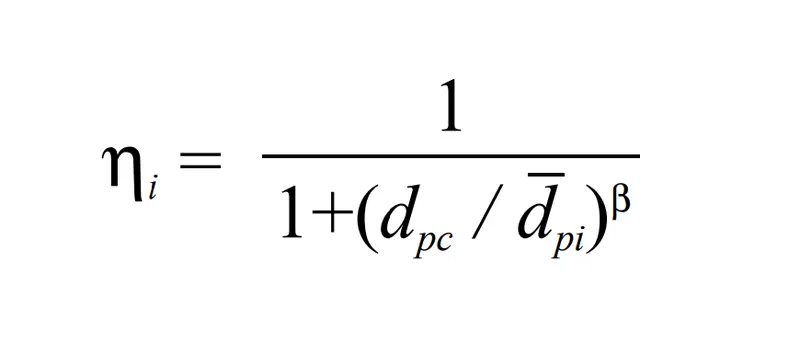
Where,
`d_"pc"` = 50% cut size and is calculated as,
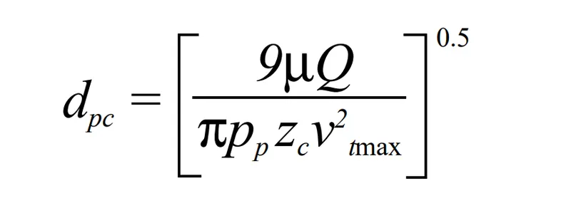
"`beta`" is the slope parameter and "`d_"pi"`" is the particle diameter.
2. LI AND WANG MODEL
The Li and Wang model includes particle bounce or re-entrainment and turbulent diffusion at the cyclone wall. A two-dimensional analytical expression of particle distribution in the cyclone is obtained.
The expression of the collection efficiency for a particular particle size is given by,
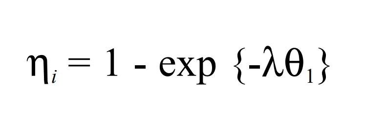
Where,
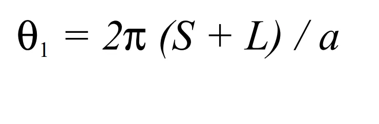
And,
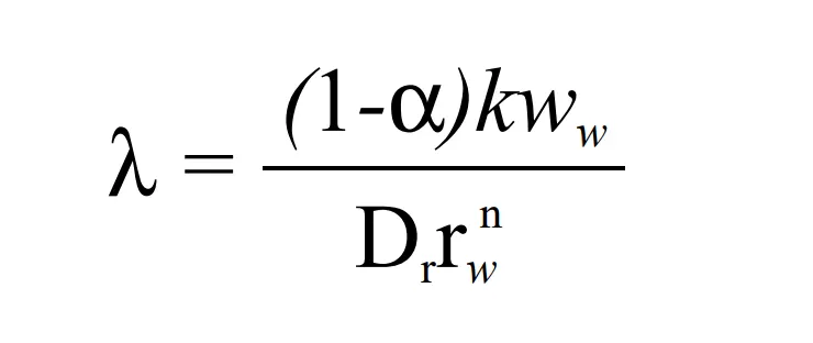
3. KOCH AND LICHT MODEL
Koch and Licht collection theory recognized the inherently turbulent nature of cyclones and the distribution of gas residence times within the cyclone. Koch and Licht describe particle motion in the entry and collection regions.
A force balance and an equation on the particles collection yields the grade efficiency `η_i`.
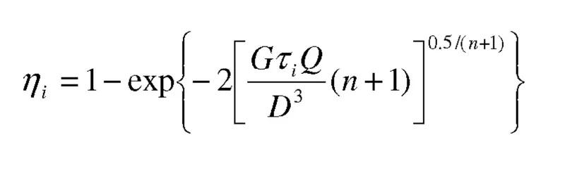
Where,
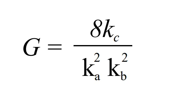
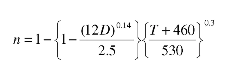
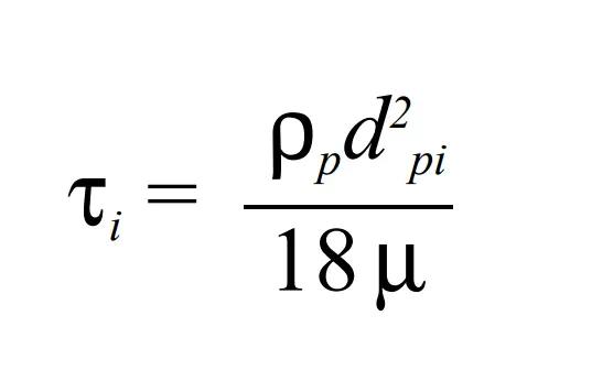
"`G`" is a factor related to the configuration of the cyclone, "`n`" is related to the vortex and "`tau`" is the relaxation term.
4. LAPPLE MODEL
Lapple model was developed based on force balance without considering the flow resistance. Lapple assumed that a particle entering the cyclone is evenly distributed across the inlet opening. The particle that travels from inlet half width to the wall in the cyclone is collected with 50% efficiency.
The efficiency of collection of any size of particle is given by,
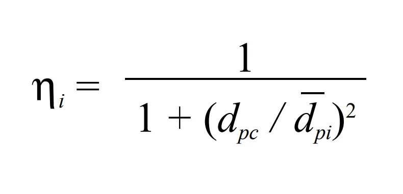
Where,
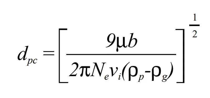
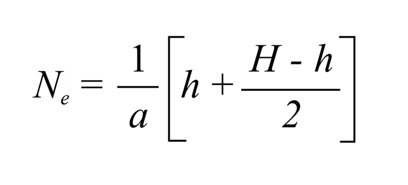
"`N_e`" is the number of revolutions and "`d_"pc"`" is the 50% cut diameter.
CASE STUDY :
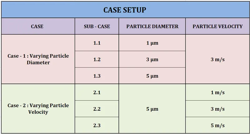
In this simulation, we are going to carry out 2 case studies, wherein we vary the particle size in the first case and we vary the particle velocity in the second case. We are going to have 3 sub-cases each, representing 3 different values for which we carry out the case study. The case setup is as shown.
SIMULATION PROCEDURE :
For this challenge, we carry out the simulation procedure in 5 steps namely,
- Geometry
- Meshing
- Setup
- Solution
- Results
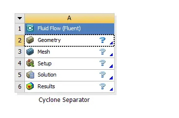
The geometry, meshing and general setup steps are the same for both the cases and their sub-cases.
1. GEOMETRY
The first step in geometry preparation is importing the step file of the geometry into the ANSYS SpaceClaim software. The model file of the cyclone separator is as shown.
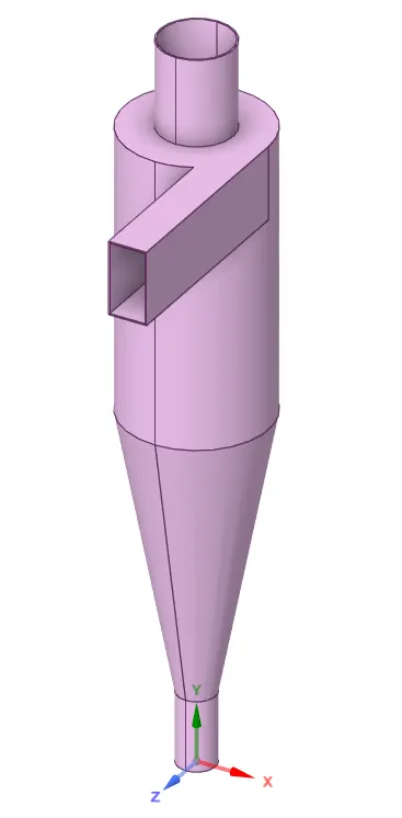
For this geometry, we then perform volume extraction so as to extract the fluid volume surface. We do so using the volume extract function in the prepare geometry tab.
We select the inlet edge of the geometry through which the flue gases or mixture enter, the outlet at the top through which air and the lighter particles escape and also the outlet at the bottom into which the larger particulate matter drop down.
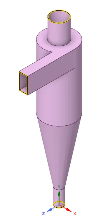
The fluid volume extraction of the geometry is as shown.
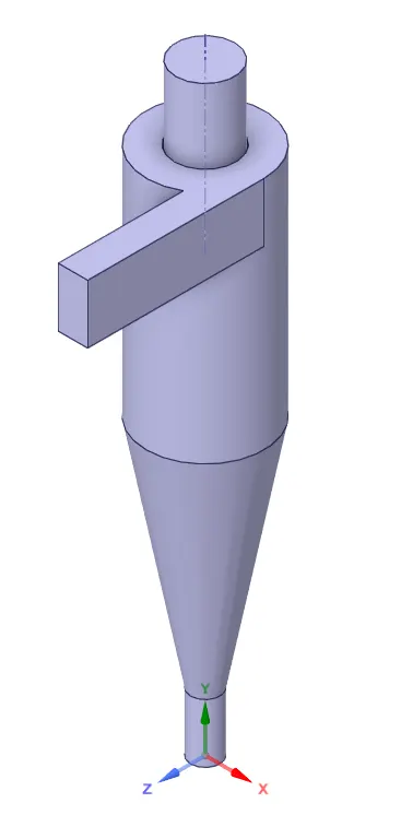
Finally, we suppress physics for the outer geometry to make sure that only the fluid volume is imported into meshing.
2. MESHING
After loading the extracted geometry into meshing, we first create named selections of the inlet and outlet faces as follows.
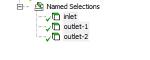
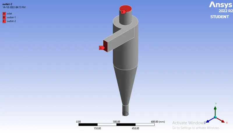
Next, we generate the mesh for an element size of 10 mm to obtain the following meshed model.
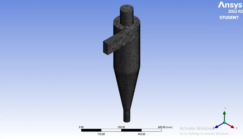
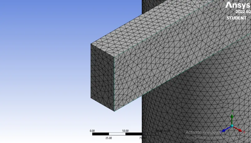
The number of meshed cells on the inlet face represent how many particles enter into the cyclone separator, through the inlet region.
4. SETUP
In this step, we are going to provide the necessary parameters to setup the simulation as per the provided data and required output results.
General Setup :
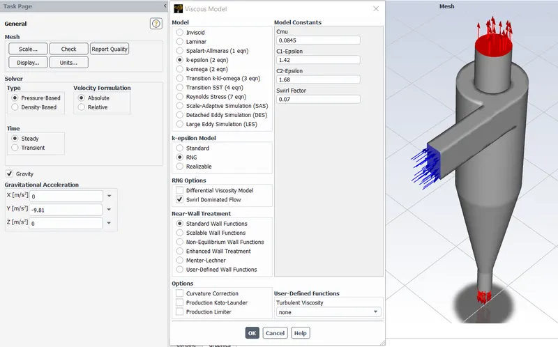
- We use a pressure – based solver with absolute velocity formulation for this simulation.
- We consider steady state time management with gravity enabled in the negative Y – axis for a value of 9.81 m/s.
- We use the RNG k – epsilon turbulence model, which is a modification of the standard k – epsilon model that enhances accuracy of swirling flows. Thereby we enable the swirl dominated flow.
Discrete Phase Modelling :
For this simulation, we use the discrete phase modelling. DPM is employed when we want to represent solid particles in a gas or liquid, such as liquid droplets in a gas and bubbles in a liquid.
Interaction :
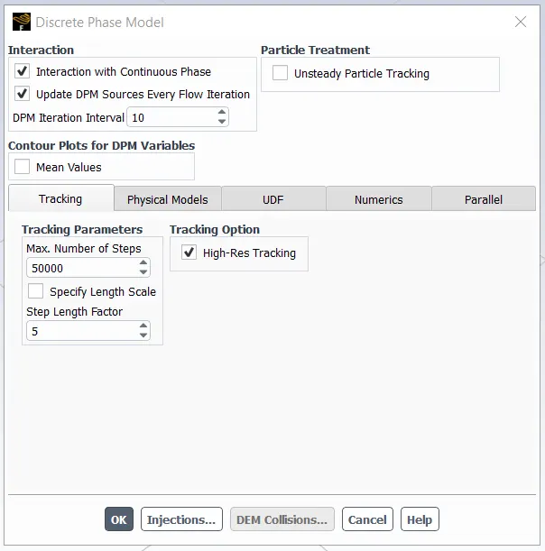
- We enable the option of “interaction with continuous phase”, which enables coupled flow of the mixture. This means that there is interaction between the discrete phase and the continuous phase.
- We update the DPM sources every flow iteration at an interval value of 10, which enables us to track the particle source terms at a frequency of 10 intervals.
Tracking Parameters :
- We specify the maximum number of steps as 50,000. This value is the number of time-steps used to compute the particle trajectory. If this limit is exceeded, which may be due to a particle trapped in the re-circulation region, then Fluent automatically cancels reporting of the trajectory and thereby preventing the particle from being tracked infinitely.
- We provide a step length factor value of 5. This option is used to control the time-step size. While calculating time-step size using step length factor, the larger the step length factor, the smaller the time-step value, which thereby increases accuracy of the trajectory.
Boundary Conditions :
As per the boundary condition data provided in the challenge, we specify the conditions as follows.
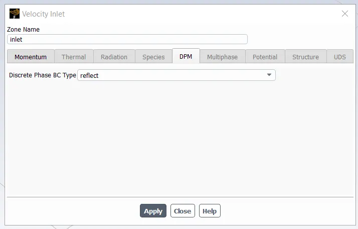
1. Inlet
DPM BC Type = Reflect
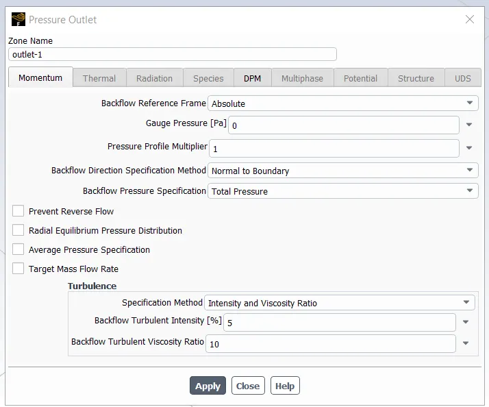
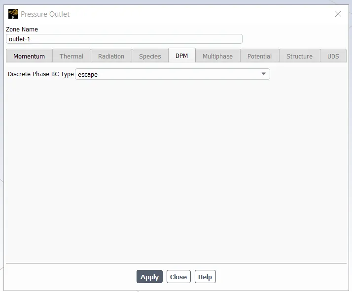
2. Outlet – 1 (Top)
Gauge Pressure = 0 Pa
DPM BC Type = Escape
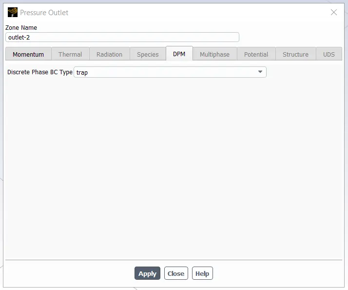
3. Outlet – 2 (Bottom / Dustbin)
Gauge Pressure = 0 Pa
DPM BC Type = Trap
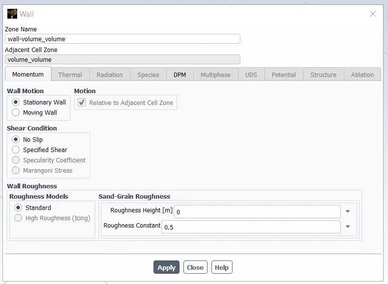
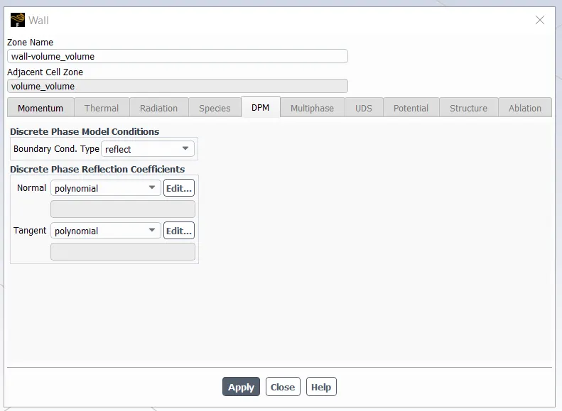
4. Walls
Wall Motion = Stationary Wall
Shear Condition = No Slip
DPM BC Type = Reflect
4. SOLUTION
In this step, we define a few parameters necessary to run the calculations.
Solution Methods :
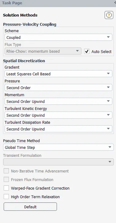
The spatial discretization schemes for turbulent kinetic energy and turbulent dissipation rate are changed to the second order upwind scheme, as it is more accurate.
Initialization :
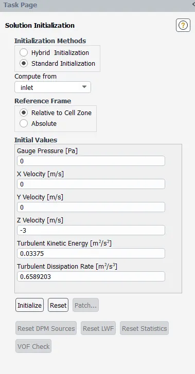
In this step, we use the standard initialization method to compute the values from the inlet. The initial values are set to the default values as shown. We then initialize the simulation and carry out the calculations.
CASE – 1 : VARYING THE PARTICLE SIZE
In this case study, we are going to be varying the particle diameter by keeping the particle velocity constant, so as to observe the effects caused by the variation on the output results. We are going to simulate 3 sub-cases for this study as follows.
Case – 1.1 : Particle Diameter = 1 µm
We are going to setup this case for a particle diameter of 1 µm, while maintaining the particle velocity at 3 m/s. We first complete the general setup of the simulation as shown above.
Injection :
During the discrete phase modelling, we create an injection method, which specifies the injection of the discrete phase particles onto the continuous phase.
- We specify the injection type as surface injection and we apply it for the inlet surface.
- The particle type is selected as “inert”, which is a discrete phase element (particle, droplet or bubble) that obeys the force balance equation and is subjected to heating or cooling.
- The particle material is selected as anthracite, which is a hard variety of coal that contains relatively pure carbon.
- Next, we provide the value of velocity, which acts normal to the surface selected. Thereby, we provide a velocity value of 3 m/s along the X – axis.
- Finally, we provide the diameter of the particle, which in this sub-case is 1 µm.
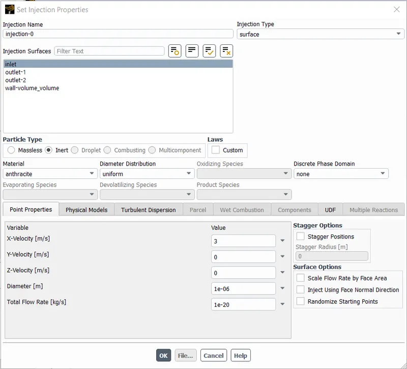
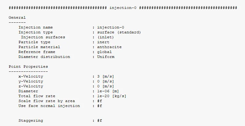
The general and point properties of injection are as follows.
Boundary Conditions :
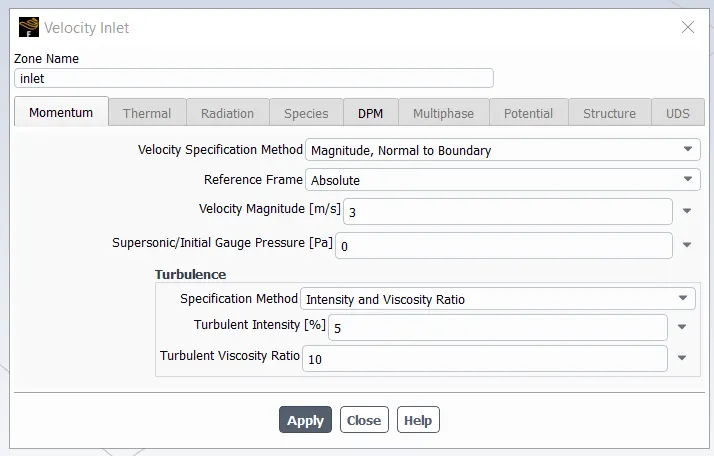
Along with the general boundary condition setup as previously shown, the particle velocity at the inlet is provided as 3 m/s and the DPM BC type set to reflect.
We then standard initialize the simulation, to compute the values from the inlet and we run the simulation for 600 iterations so as to obtain the following results.
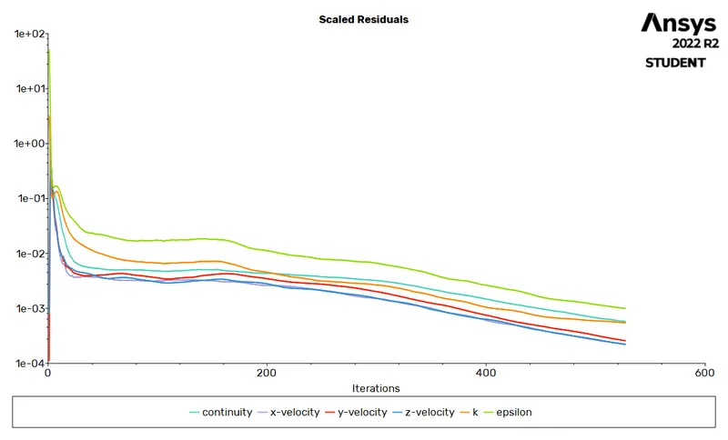
Residuals Plot :
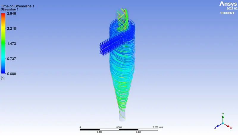
Particle Time Data :
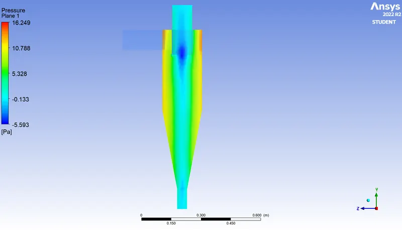
Pressure Contour :
Vortex Core Region Contour :
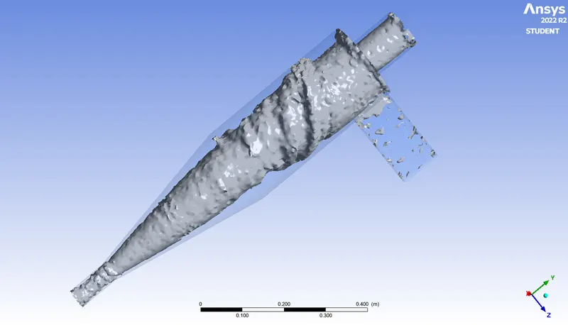
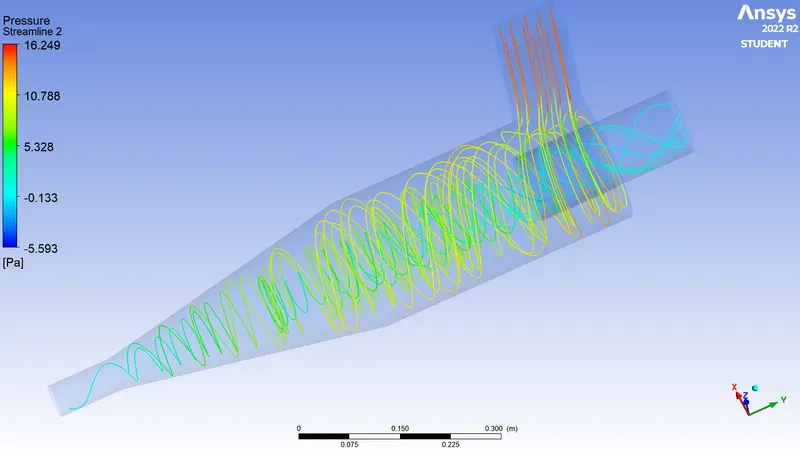
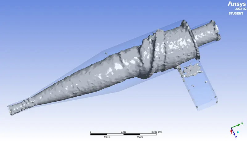
Vortex displayed in the form of streamlines, representing the low pressure vortex region created in the central region of the cyclone separator.
Particle Track & Separation Efficiency :
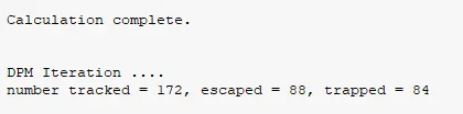
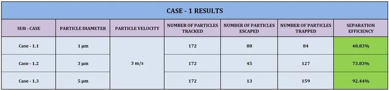
Total number of particles tracked at inlet = 172
Total number of particles escaped from top outlet = 88
Total number of particles trapped at dustbin = 84
`"Separation Efficiency" = "Trapped Particles" / "Tracked Particles" xx 100`
`=` `84 / 172 xx 100`
Therefore, Separation Efficiency = 48.83 %
Final Solution Animation :
Case – 1.2 : Particle Diameter = 3 µm
We first perform the general setup for this case, for a particle diameter of 3 µm, while maintaining the particle velocity at 3 m/s, being the same as that of the previous sub-case.
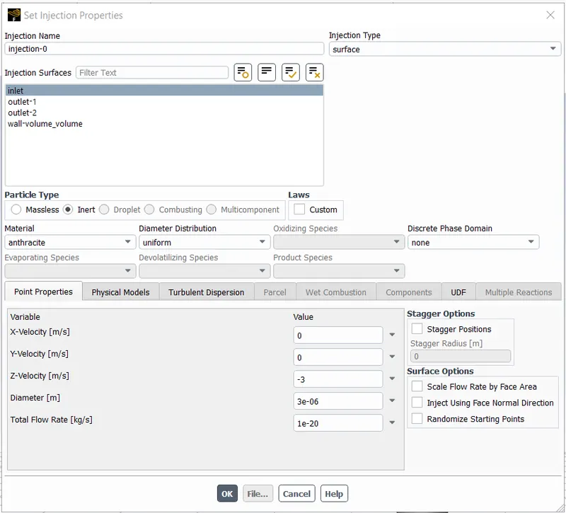
By providing the respective boundary conditions which are the same as of that of the previous sub-case, we obtain the point properties as follows.
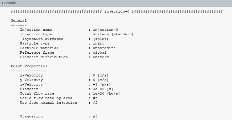
By standard initializing the simulation to compute the values from the inlet and running it for 600 iterations, we obtain the following results.
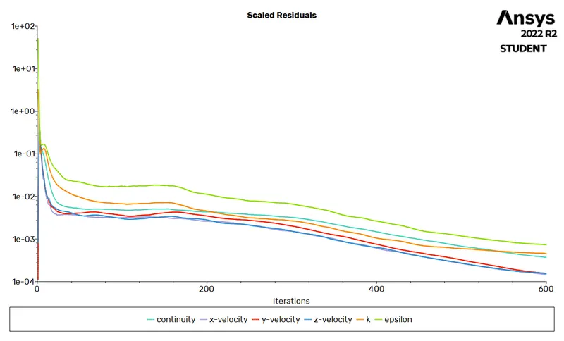
Residuals Plot :
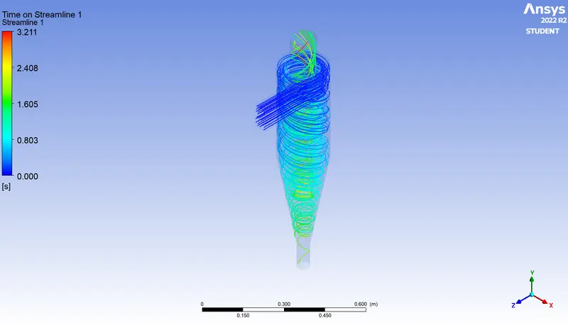
Particle Time Data :
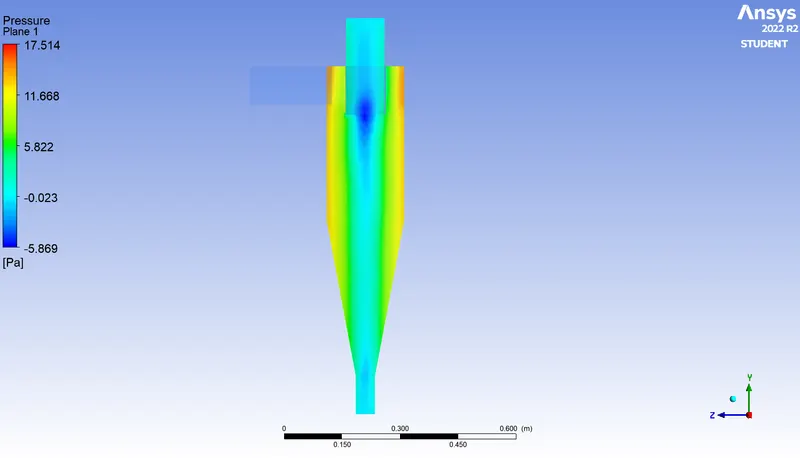
Pressure Contour :
Vortex Core Region Contour :
Particle Track & Separation Efficiency :
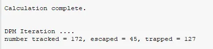
Total number of particles tracked at inlet = 172
Total number of particles escaped from top outlet = 45
Total number of particles trapped at dustbin = 127
`"Separation Efficiency" = "Trapped Particles" / "Tracked Particles" xx 100`
`=` `127 / 172 xx 100`
Therefore, Separation Efficiency = 73.83 %
Final Solution Animation :
Case – 1.3 : Particle Diameter = 5 µm
We first perform the general setup for this case, with all the parameters being the same as that of the previous two sub-cases, for a particle diameter of 5 µm and particle velocity at 3 m/s.
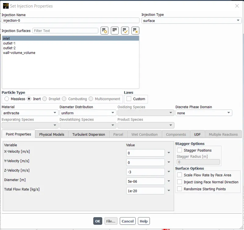
The particle point properties are as displayed.
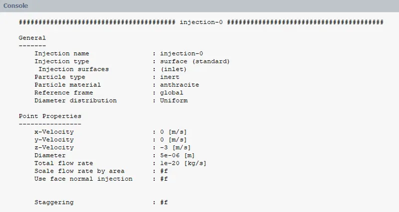
Thereby, standard initializing the simulation and running it for 600 iterations, we obtain the following results.
Residuals Plot :
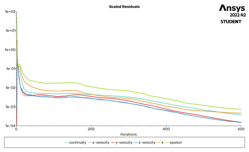
Particle Time Data :
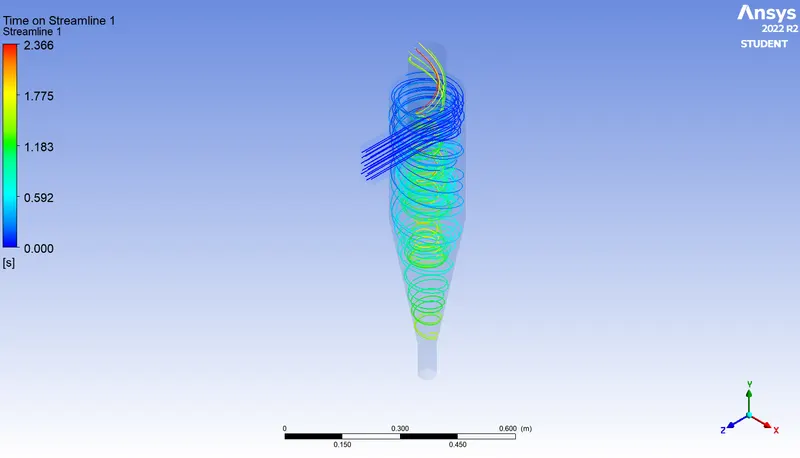
Pressure Contour :
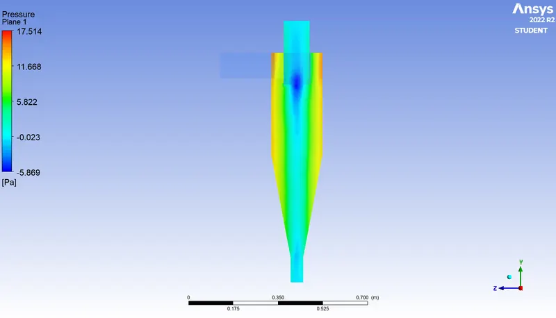
Vortex Core Region Contour :
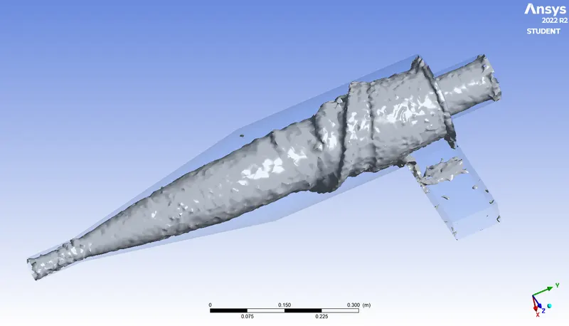
Particle Track & Separation Efficiency :
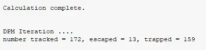
Total number of particles tracked at inlet = 172
Total number of particles escaped from top outlet = 13
Total number of particles trapped at dustbin = 159
`"Separation Efficiency" = "Trapped Particles" / "Tracked Particles" xx 100`
`=` `159 / 172 xx 100`
Therefore, Separation Efficiency = 92.44 %
Final Solution Animation :
Final Results :
The final result comparison of the three sub – cases is represented as follows.
CASE – 2 : VARYING PARTICLE VELOCITY
In this case study, we are going to be varying the particle inlet velocity between a range of 1 m/s to 5 m/s to observe its effects on the separation efficiency and pressure drop of the cyclone separator. We are going to carry out 3 sub – cases representing the various values of inlet particle velocity by maintaining a constant particle diameter of 5 µm.
Case – 2.1 : Particle Inlet Velocity = 1 m/s
In this sub – case study, first we are going to carry out the common general setup of the simulation as we have in all the previous steps. Next, for a constant particle size of 5 µm, we are going to provide the particle inlet velocity as 1 m/s so as to observe its effects.
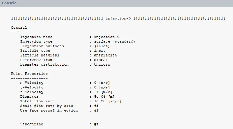
The injection properties are as shown and is common for all 3 sub – cases.
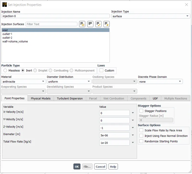
The particle point properties are represented as follows.
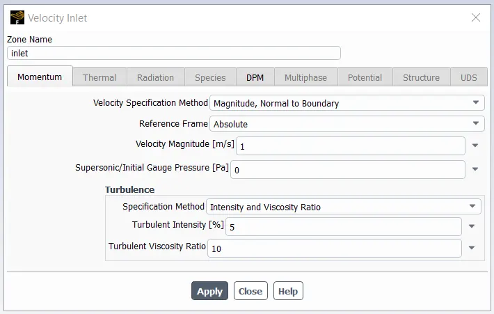
Boundary Conditions :
We provide the boundary conditions of velocity magnitude at the inlet surface to be 1 m/s.
We define the respective pressure plots, so as to measure the pressure difference obtained at the inlets and the outlets. We then standard initialize the simulation as follows.
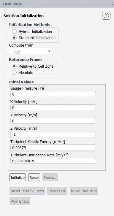
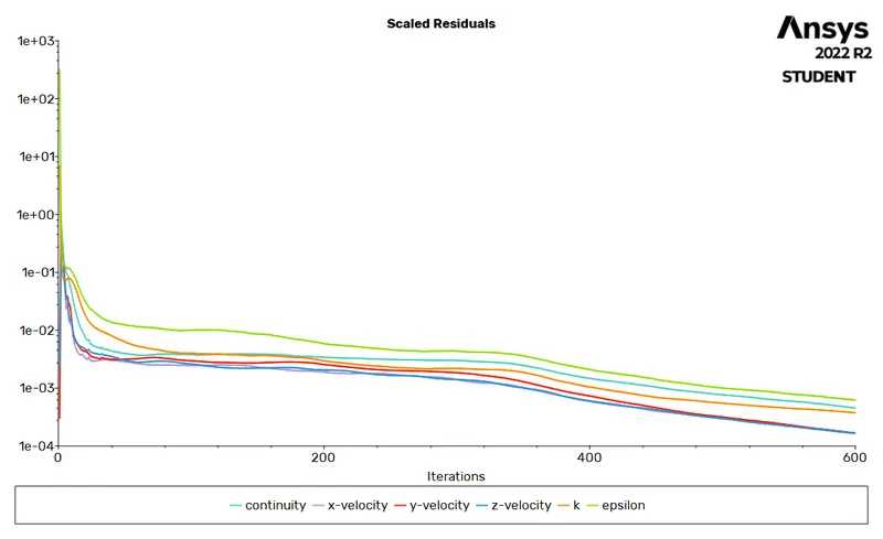
By running the simulation for 600 iterations with the above mentioned conditions, we obtain the following plots and results.
Residuals Plot :
Pressure Contour :
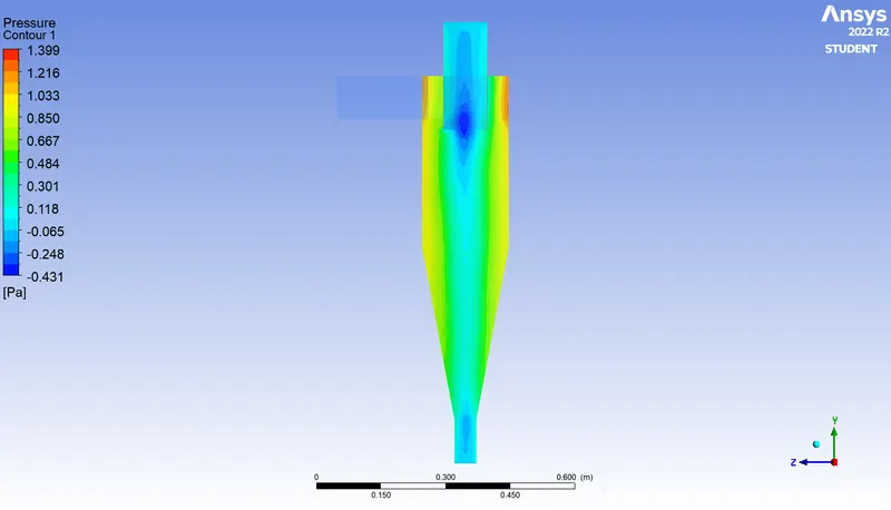
From the above contour, we can observe that the pressure of the vortex region created at the mid – section of the separator is comparatively less and thereby, the number of particles brought up by the vortex low pressure region or escaped particles is less, due to the low velocity.
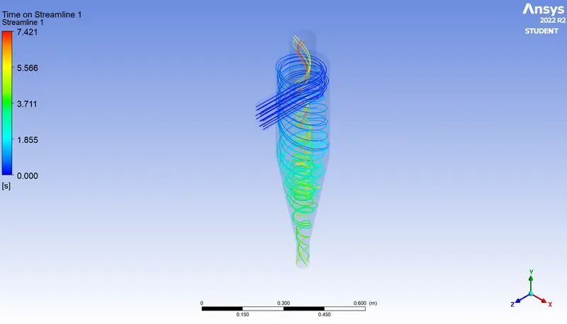
Particle Track :
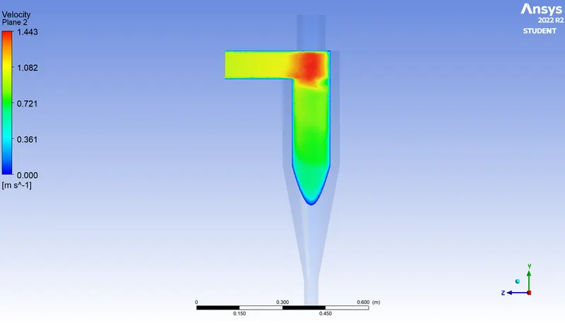
Velocity Contour :
The velocity contour of the particles flowing in from the inlet surface is as shown below. The blue region adjacent to the walls represent the no-slip condition of the walls.
Pressure Plots :
The area – weighted average pressure plots obtained at the inlet and outlets of the simulation are as shown.
1. Inlet Pressure
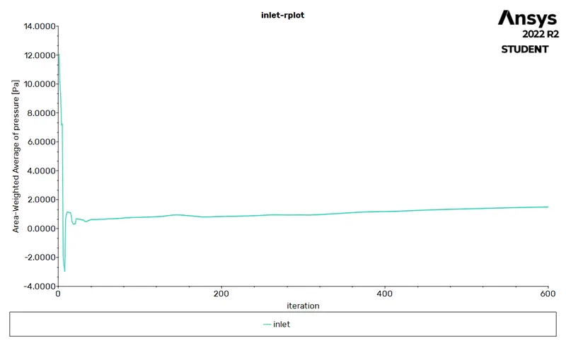
Inlet Pressure = 1.5385 Pa
2. Outlet – 1 Pressure (Top)
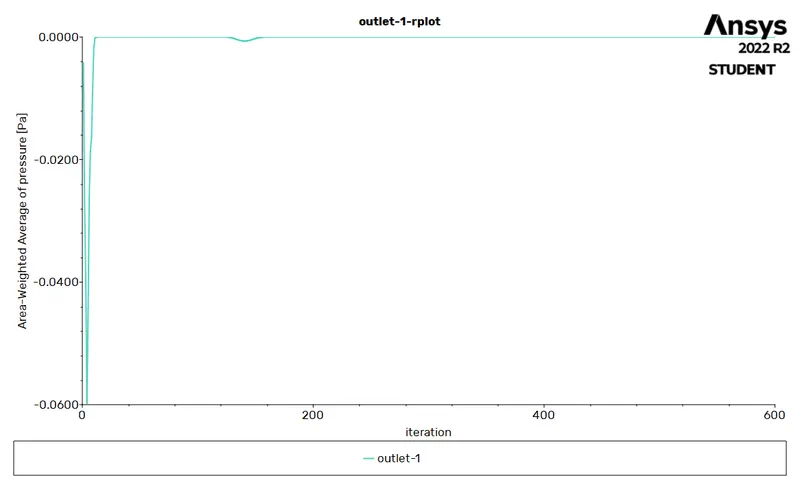
Outlet – 1 Pressure = 0.0002 Pa
3. Outlet – 2 Pressure (Bottom)
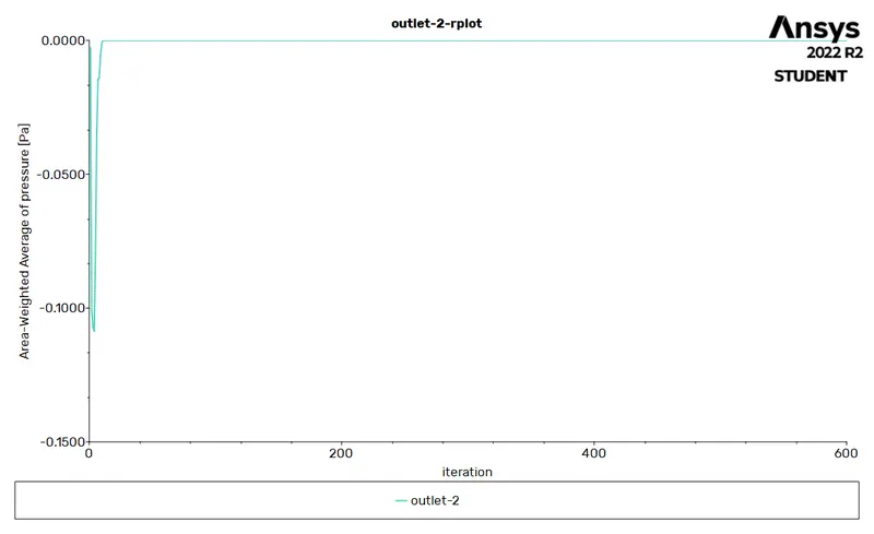
Outlet – 2 Pressure = 0.0005 Pa
The pressure drop is calculated as the difference between the inlet pressure and outlet pressure.
`"Pressure"` `"Drop"_1` = `"Inlet Pressure"` – `"Outlet"_1``" Pressure"`
`= 1.5385` `– 0.0002`
`therefore` `Delta P _ ("inlet" – "outlet"_1)` `= 1.5383` `Pa`
`"Pressure"` `"Drop"_2` = `"Inlet Pressure"` – `"Outlet"_2``" Pressure"`
`= 1.5385` `– 0.0005`
`therefore` `Delta P _ ("inlet" – "outlet"_2)` `= 1.538` `Pa`
Case – 2.2 : Particle Inlet Velocity = 3 m/s
For this sub-case study, we are going to increase the particle inlet velocity to 3 m/s for the same simulation conditions and particle diameter of 5 µm.
The particle injection properties are defined as,
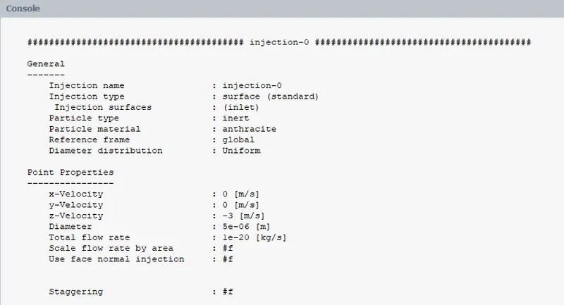
With reference to the above conditions, we provide the velocity magnitude value at the inlet as 3 m/s.
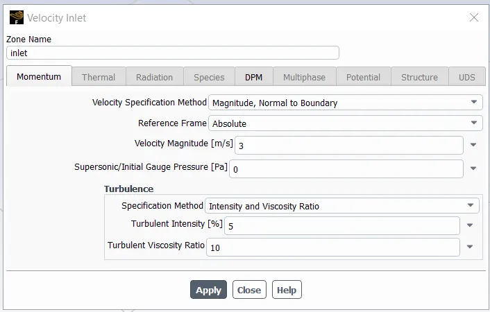
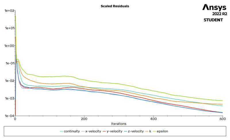
Finally, we standard initialize the simulation and run it for 600 iterations to obtain the following results.
Residuals Plot :
Pressure Contour :
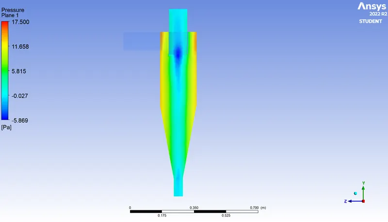
From the above contour, we can observe that the pressure of the vortex region is significantly higher than the previous sub-case and thereby, the number of particles brought up by the vortex low pressure region or escaped particles is higher.
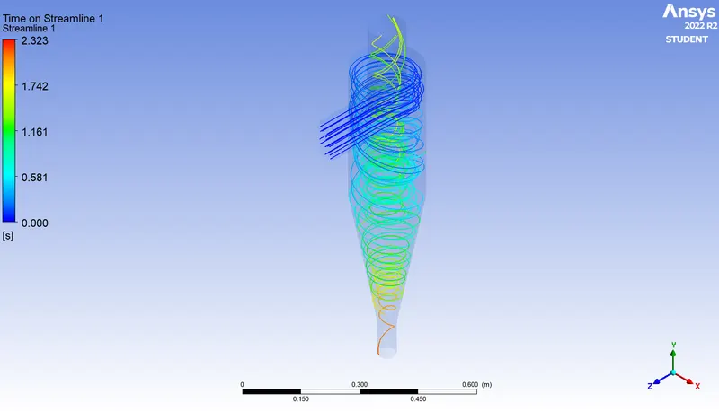
Particle Track :
Velocity Contour :
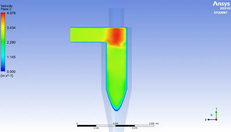
The velocity contour plot is represented as follows, consisting of a no-slip condition along the geometry walls.
Vortex Region :
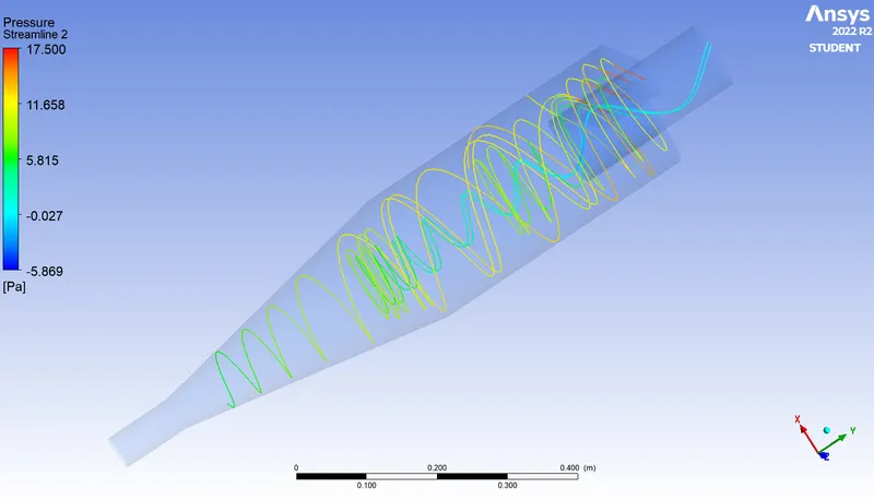
The low pressure vortex created inside the separator is as shown below.
Pressure Plots :
The area – weighted average pressure plots obtained at the inlet and outlets of the simulation are as shown.
1. Inlet Pressure
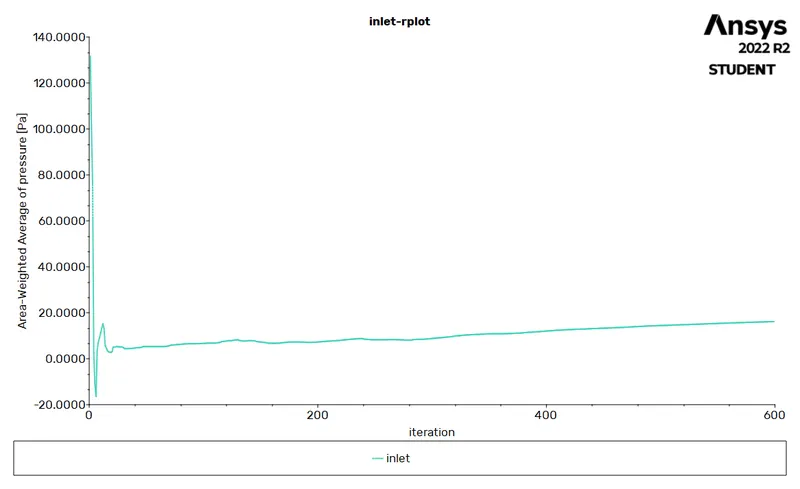
Inlet Pressure = 16.3506 Pa
2. Outlet – 1 Pressure (Top)
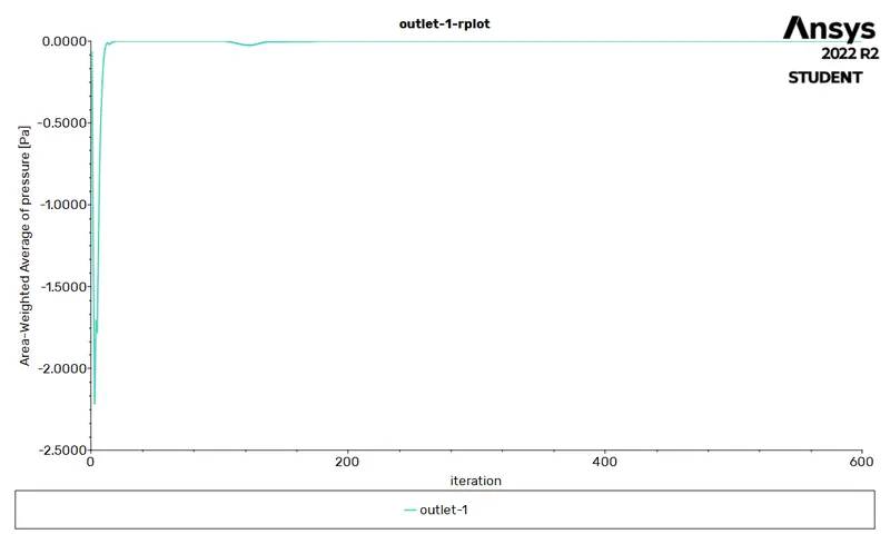
Outlet – 1 Pressure = - 0.0045 Pa
3. Outlet – 2 Pressure (Bottom)
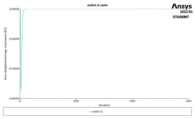
Outlet – 2 Pressure = - 0.0107 Pa
The pressure drop is calculated as the difference between the inlet pressure and outlet pressure.
`"Pressure"` `"Drop"_1` = `"Inlet Pressure"` – `"Outlet"_1``" Pressure"`
`= 16.3506` `+ 0.0045`
`therefore` `Delta P _ ("inlet" – "outlet"_1)` `= 16.3551` `Pa`
`"Pressure"` `"Drop"_2` = `"Inlet Pressure"` – `"Outlet"_2``" Pressure"`
`= 16.3506` `+ 0.0107`
`therefore` `Delta P _ ("inlet" – "outlet"_2)` `= 16.3613` `Pa`
Case – 2.3 : Particle Inlet Velocity = 5 m/s
For this sub-case study, we further increase the particle inlet velocity to 5 m/s for the particle diameter of 5 µm to observe the results.
The particle injection properties are defined as,
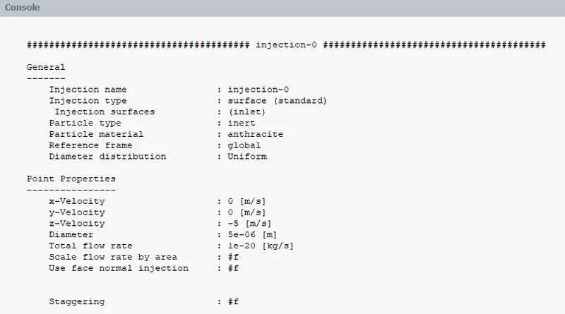
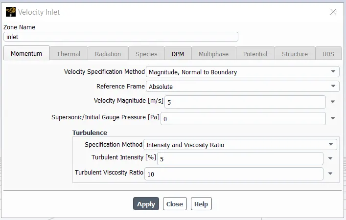
The inlet boundary conditions are provided as follows.
Finally, we standard initialize the simulation to compute it from the inlet, to obtain the initial values as follows.
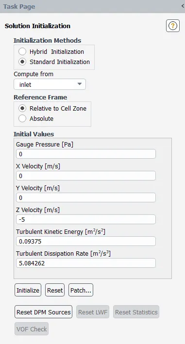
We run the simulation for 600 iterations so as to obtain the following results.
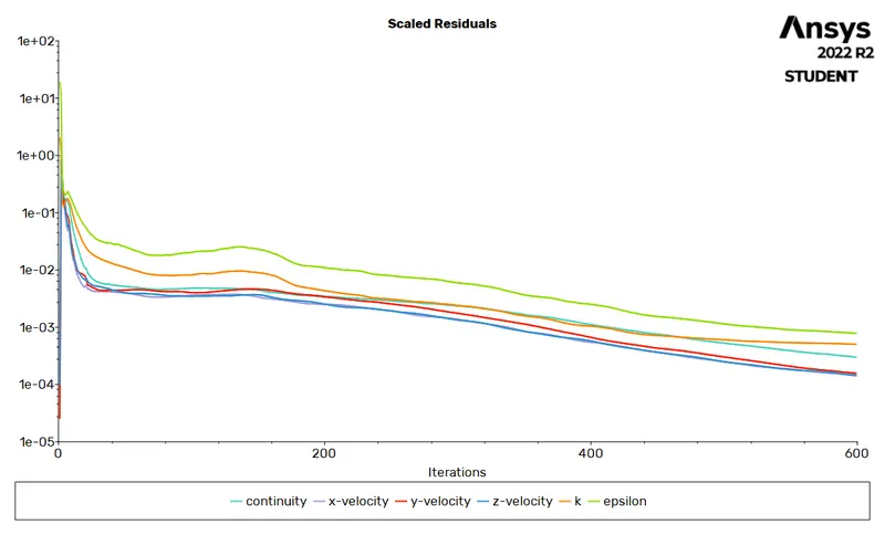
Residuals Plot :
Pressure Contour :
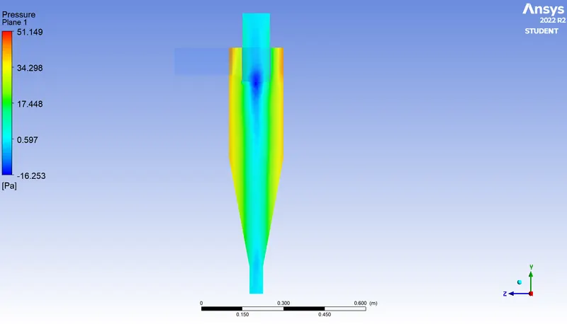
From the above contour plot, we can observe that the negative pressure produced in the vortex core region is higher as well as the total pressure, due to the increase in velocity.
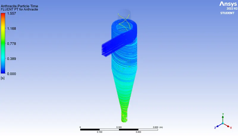
Particle Track :
Velocity Contour :
The velocity contour plot is represented as follows, consisting of a no-slip condition along the geometry walls.
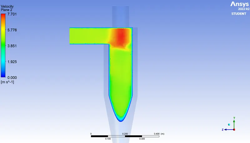
Vortex Region :
The visual representation of a single particle which is re-circulated inside the vortex core region and escapes out through the top outlet is as shown below.
Pressure Plots :
The area – weighted average pressure plots obtained at the inlet and outlets of the simulation are as shown.
1. Inlet Pressure
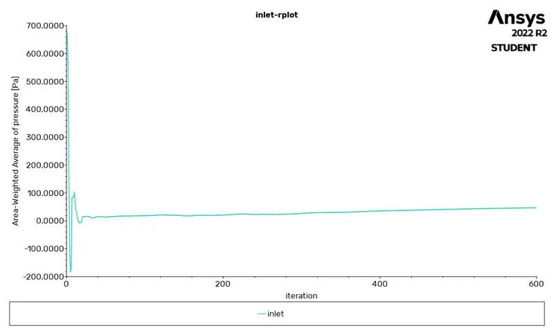
Inlet Pressure = 49.4565 Pa
2. Outlet – 1 Pressure (Top)
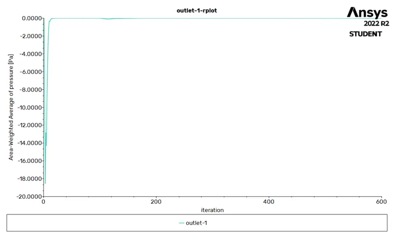
Outlet – 1 Pressure = - 0.0362 Pa
3. Outlet – 2 Pressure (Bottom)
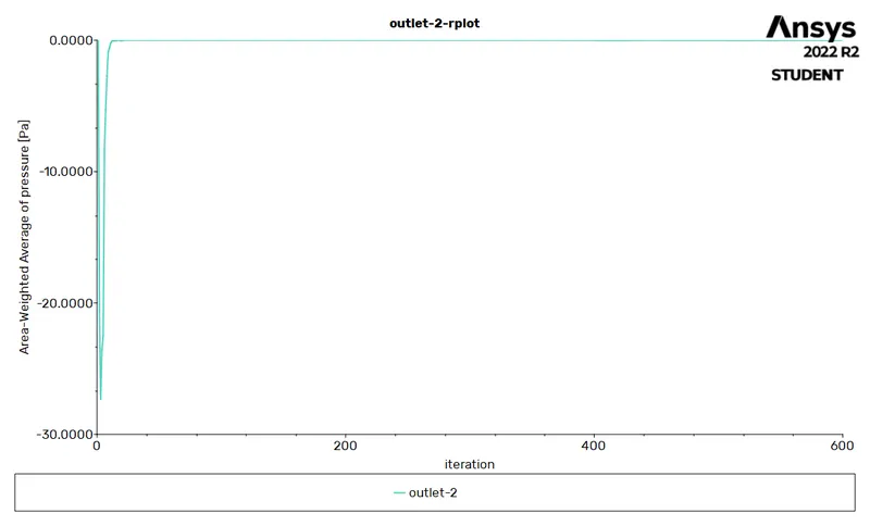
Outlet – 2 Pressure = 0.0543 Pa
The pressure drop is calculated as the difference between the inlet pressure and outlet pressure.
`"Pressure"` `"Drop"_1` = `"Inlet Pressure"` – `"Outlet"_1``" Pressure"`
`= 49.4565` `+ 0.0362`
`therefore` `Delta P _ ("inlet" – "outlet"_1)` `= 49.4927` `Pa`
`"Pressure"` `"Drop"_2` = `"Inlet Pressure"` – `"Outlet"_2``" Pressure"`
`= 49.4565` `- 0.0543`
`therefore` `Delta P _ ("inlet" – "outlet"_2)` `= 49.4022` `Pa`
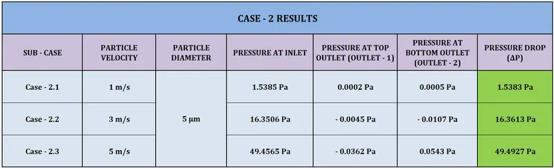
Final Results :
The final result comparison of the three sub – cases and their details is represented as follows.
CONCLUSIONS :
The simulation has been successfully run for both the cases and their sub-cases and their respective plots and contours have been obtained as shown. The effects due to the variation of particle diameter size as well as the particle velocity, on the separation efficiency have been successfully studied and compared.
From the results obtained from the first case study, wherein the particle size has been varied. We can observe that for a constant inlet velocity, as the particle size increases, the outlet or separation efficiency of the cyclone separator also increases. This is due to the fact that, if the particle size is too small, they tend to get carried upwards due to the low pressure vortex created in the middle and they escape out, along with the flue gases as they are less denser. On the contrary, if the particle sizes are larger, the re-circulating vortex tends to not have that great of an effect on these particles and they settle down and collect into the bottom outlet or dustbin. Therefore, the particle size is directly proportional to the separation efficiency and greater the particle size, higher the separation efficiency. The variation of particle size has no significant impact on the pressure drop of the system.
In the second case study, for a constant particle size, we vary the inlet velocity of the particles. From the results obtained, we can observe that for a lower velocity value, the vorticity effects on the particles are considerably less, leading to a large number of particles just dropping straight down from the inlet without any circulation. We can also concur that, with the increase in particle inlet velocity, we obtain larger differences in pressure or pressure drop between the inlet and outlet regions. Therefore, higher the inlet velocity of the particles, greater the pressure difference or pressure drop.
A high pressure region is formed near the walls of the cyclone separator due to the formation of the outer vortex and thereby leading to a low pressure region creation at the middle of the geometry, which we refer to as the vortex core region. This vortex tends to re-circulate the less denser particles up and out through the top outlet.