Week 7 - Simulation of a 1D Super-sonic nozzle flow simulation using Macormack Method

AIM :

To simulate the isentropic flow through a Quasi 1-D Subsonic - Supersonic Nozzle.

OBJECTIVES :

1. Derive the conservative and non-conservative forms of the Quasi 1-D Subsonic – Supersonic Nozzle governing equations and solve them using the MacCormack’s technique.
   
   
   
2. Determine the steady-state temperature distribution for the flow-field variables and investigate the difference between the two forms of governing equations by comparing their solutions.
   
   
   
3. To write a MATLAB program to represent the following plots,
   i.) Steady-state distribution of primitive variables inside the nozzle.
   ii.) Time-wise variation of the primitive variables.
   iii.) Variation of Mass flow rate distribution inside the nozzle at different time steps during the time-marching process.
   iv.) Comparison of Normalized mass flow rate distributions of both forms.
   
   
   
4. Perform a grid independence test on the solution and explain all our findings.

INTRODUCTION :

In this context, we are going to be solving the two forms of the Quasi 1-D Steady Subsonic – Supersonic Nozzle flow, being the conservative and non-conservative forms.

Quasi 1-D Flow :

A quasi-one-dimensional flow is one in which all variables vary primarily along one direction, say x. That means that the cross-section is allowed to vary smoothly but flow quantities varies in one direction only. We will further assume steady-state flow, which means that unsteady terms will be zero.

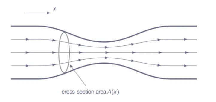
Even though the area of nozzle changes as a function of distance along nozzle (i.e, flow is 2-D), we assume that flow properties are uniform along given section (i.e, flow varies only along x-axis and the flow along y-axis does not vary). These types of flows are defined as Quasi 1-D.

Subsonic and Supersonic Flows :

Subsonic flow refers to the motion of a fluid whose velocity is lesser than the speed of sound.

`M < 1`

Supersonic flow refers to the motion of a fluid whose velocity is greater than the speed of sound.

`M > 1`

Where, M = Mach Number (Speed of Sound)

Note : 1 Mach = Speed of Sound ( 1 is the multiplication factor )

= 343 m/s or 761.2 mph or 1225 kmph

Mach Number :

It is the ratio of speed of a body to speed of sound in the surrounding medium.

`M = u/c`

Where,

`M` = Local Mach number

`u` = Local flow velocity with respect to the boundaries

`c` = Speed of sound in the medium

MacCormack’s Method :

It is an explicit finite – difference technique which is second order accurate in both space and time. In MacCormack’s method, we are splitting the time marching solution into 2 phases.

1. Predictor Step :
   We initially start with the initial conditions and from these conditions, we calculate the values of the next time step, called the predictor timestep. In this timestep, we calculate the L.H.S quantities (time derivatives) and we represent it in a general form as `(delf)/(delt_p)`, where ‘`f` ’ can be density, velocity or temperature.
   
   
   Once we have the predictor step, we are going to perform a solution update. It means that, from the predictor time derivatives, we are going to compute the value of ‘`f` ’.
   
   `f^ast = f_("initial") + (delf)/(delt_p).Deltat`
   
   
   
   
   
   
   
2. Corrector Step :
   With the new solution '`f^ast` ' from solution update, we calculate the corrector step `(delf^ast)/(delt_c)`.
   
   
   Finally, we calculate a new time derivative called average time derivative, which is the arithmetic mean of predictor step and corrector step values.
   
   `((delf)/(delt))_("avg") = 1/2((delf)/(delt_p) + (delf)/(delt_c))`
   
   Once we have this new time derivative, we will be able to compute actual value of '`f` ' in the next time step.
   
   `f^"2nd time step" = f_"initial" + ((delf)/(delt))_(avg) . Deltat`

The difference between predictor and corrector step is that, in predictor step – we use Forward Differencing for space terms and in corrector step, we use Backward Differencing.

DIAGRAM :

Considering the steady, isentropic flow through a convergent – divergent nozzle.

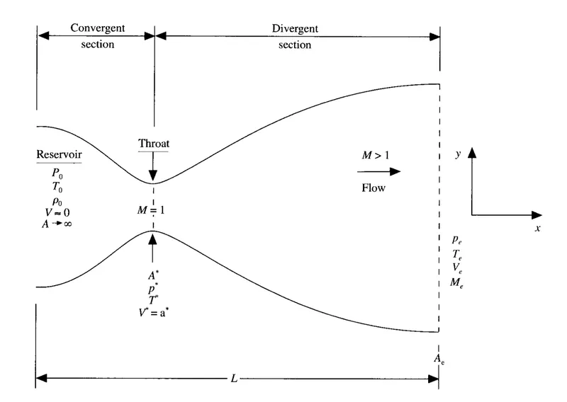
The flow at the inlet of the nozzle comes from a reservoir where the pressure and temperature are denoted by `P_o` and `T_o`, which are the stagnation values. The cross – sectional area of the reservoir is large ( `A -> infty` ) and hence the velocity is very small ( `V -> 0` ).

The flow expands isentropically to supersonic speeds at the nozzle exit, where the exit pressure, temperature, velocity and mach number are denoted by `P_e` , `T_e` , `V_e` and `M_e`. The flow is locally subsonic in the convergent section of nozzle, sonic at the throat (minimum area) and supersonic at the divergent section.

NON – CONSERVATIVE FORM :
The non- conservative form is a form of fluid flow in which the control volume moves with respect to the flow.

Governing Equations of Non - Conservative Form :

The governing equations representing the continuity equation, momentum equation and the energy equation for the non – conservative form is given by,

1. Continuity Equation
   
   `(delrho')/(delt') = -rho'(delV')/(delx') - rho'V'(del(lnA'))/(delx') - V'(delrho')/(delx')`
   
   
   
   
2. Momentum Equation
   
   `(delV')/(delt') = -V'(delV')/(delx') - 1/gamma((delT')/(delx') + (T')/(rho')(delrho')/(delx'))`
   
   
   
   
3. Energy Equation
   
   `(delT')/(delt') = -V'(delT')/(delx') - (gamma - 1).T'[(delV')/(delx') + V'(del(lnA'))/(delx')]`
   
   
   
   
4. Non – Dimensional Variables
   
   Temperature, `T' = T/(T_o)`
   
   Density, `rho' = rho/(rho_o)`
   
   Distance, `x' = x/L`
   
   Velocity, `V' = V/(a_o)`
   
   Area, `A' = A/(A^ast)`
   
   Time, `t' = t/(L/(a_o))`
   
   
   Where,
   prime ( ' ) = Dimensionless variable
   
   `T_o` = Reservoir temperature
   
   `rho_o` = Reservoir density
   
   `L` = Length of nozzle
   
   `a_o` = Speed of sound in reservoir
   
   
   
   
   
   
   

MacCormack’s Method for Non - Conservative Form :

Here, we are going to implement a finite difference MacCormack’s explicit technique to obtain the numerical solution of the governing equations.

1. Predictor Step :
   We are using forward differencing scheme for the spatial derivative terms. Further, we are going to calculate solution variant for which we obtain an intermediate solution.
   
   Discretizing the continuity, momentum and energy governing equations as follows,
   
   Continuity `->` `((delrho)/(delt))_i^t = -rho_i^t ((V_(i+1)^t - V_i^t)/(Deltax)) -rho_i^t V_i^t ((ln(A_(i+1)) - ln(A_i))/(Deltax)) - V_i^t ((rho_(i+1)^t - rho_i^t)/(Deltax))`
   
   
   
   Momentum `->` `((delV)/(delt))_i^t = -V_i^t ((V_(i+1)^t - V_i^t)/(Deltax)) - 1/gamma [(T_(i+1)^t - T_i^t)/(Deltax) + (T_i^t)/(rho_i^t) ( (rho_(i+1)^t - rho_i^t)/(Deltax))]`
   
   
   
   Energy `->` `((delT)/(delt))_i^t = -V_i^t ((T_(i+1)^t - T_i^t)/(Deltax)) - (gamma-1) T_i^t [(V_(i+1)^t - V_i^t)/(Deltax) + V_i^t((ln(A_(i+1)) - ln(A_i))/(Deltax))]`
   
   
   
   Here, for a given time "t", we are going to calculate the time derivatives `(delrho)/(delt)` , `(delV)/(delt)` and `(delT)/(delt)` , which would be the solution gradients.
   
   
   
   
   
   
   
   
2. Intermediate Solution Step :
   We are finding the primitive variables at time " `t + Deltat` " from solution gradients and old primitive variable values.
   
   `rho_i^(t+Deltat) = rho_i^t + ((delrho)/(delt))_i^t .Deltat`
   
   
   `V_i^(t+Deltat) = V_i^t + ((delV)/(delt))_i^t .Deltat`
   
   
   `T_i^(t+Deltat) = T_i^t + ((delT)/(delt))_i^t .Deltat`
   
   
   
   
   
   
   
   
3. Corrector Step :
   We first obtain a corrected value of time derivative at time “ `t+Deltat` ”. These corrected values are obtained by substituting predictor values of `rho`, `V` and `T` into R.H.S of equation and replacing spatial derivative with the backward differencing scheme.
   
   `((delrho)/(delt))_i^(t+Deltat) = -rho_i^(t+Deltat) ((V_(i)^(t+Deltat) - V_(i-1)^(t+Deltat))/(Deltax)) -rho_i^(t+Deltat). V_i^(t+Deltat) [(ln(A_(i)) - ln(A_(i-1)))/(Deltax)] - V_i^(t+Deltat) ((rho_(i)^(t+Deltat) - rho_(i-1)^(t+Deltat))/(Deltax))`
   
   
   
   `((delV)/(delt))_i^(t+Deltat) = -V_i^(t+Deltat) ((V_(i)^(t+Deltat) - V_(i-1)^(t+Deltat))/(Deltax)) - 1/gamma [(T_(i)^(t+Deltat) - T_(i-1)^(t+Deltat))/(Deltax) + (T_i^(t+Deltat))/(rho_i^(t+Deltat)) ( (rho_(i)^(t+Deltat) - rho_(i-1)^(t+Deltat))/(Deltax))]`
   
   
   
   `((delT)/(delt))_i^(t+Deltat) = -V_i^(t+Deltat) ((T_(i)^(t+Deltat) - T_(i-1)^(t+Deltat))/(Deltax)) - (gamma-1). T_i^(t+Deltat) [(V_(i)^(t+Deltat) - V_(i-1)^(t+Deltat))/(Deltax) + V_i^(t+Deltat)((ln(A_(i)) - ln(A_(i-1)))/(Deltax))]`
   
   
   
   
   
   
   
   
4. Final Solution Step :
   We are going to calculate average value of time derivatives, which are obtained from the arithmetic mean of predictor and corrector step. This allows us to obtain the final values of `rho`, `V` and `T` at time `t+Deltat`.
   
   `((delrho)/(delt))_(avg) = 1/2[((delrho)/(delt))_i^t + ((delrho)/(delt))_i^(t+Deltat)]`
   
   
   `((delV)/(delt))_(avg) = 1/2[((delV)/(delt))_i^t + ((delV)/(delt))_i^(t+Deltat)]`
   
   
   `((delT)/(delt))_(avg) = 1/2[((delT)/(delt))_i^t + ((delT)/(delt))_i^(t+Deltat)]`
   
   
   
   Therefore, the final solution values are given by,
   
   `rho_i^(t+Deltat) = rho_i^(t) + ((delrho)/(delt))_(avg).Deltat`
   
   
   `V_i^(t+Deltat) = V_i^(t) + ((delV)/(delt))_(avg).Deltat`
   
   
   `T_i^(t+Deltat) = T_i^(t) + ((delT)/(delt))_(avg).Deltat`

Initial and Boundary Conditions for Non-Conservative Form :

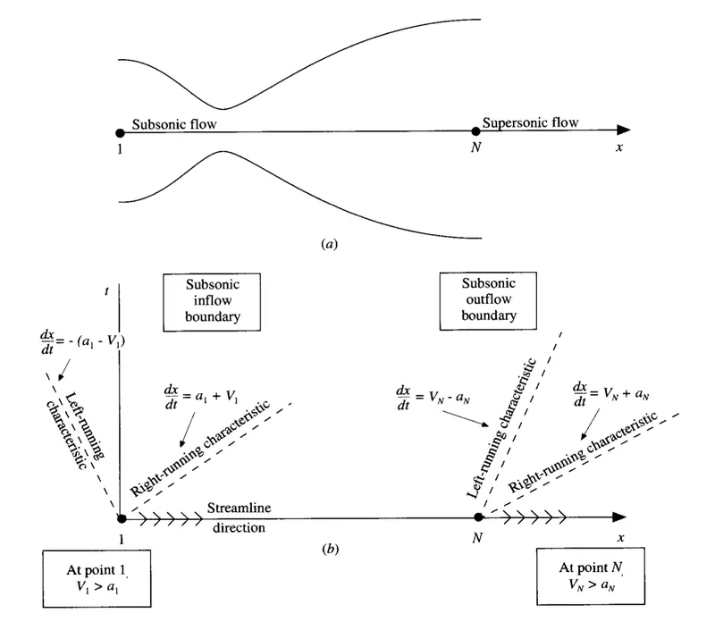
The below figure represents a convergent - divergent nozzle with an `xt` diagram sketched below it.

1. Initial Conditions
   Initializing the conditions for number of timesteps (`nt`) = 1400, number of nodes (`n`) = 31 and `i` = 1.
   
   
   `rho = 1 - 0.3146x`
   
   `T = 1 - 0.2314x`
   
   `V = (0.1 + 1.09x)T^(1/2)`
   
   `A = 1 + 2.2(x - 1.5)^2` Where, `0<=x<=3`
   
   
   
   
2. Boundary Conditions
   The inlet boundary conditions are given as,
   
   `rho_1 = 1` ; `T_1 = 1` ; `V_1 = 2V_2 - V_3`
   
   
   The outlet boundary conditions are taken as,
   
   `V_N = 2V_(N-1) - V_(N-2)`
   
   `rho_N = 2rho_(N-1) - rho_(N-2)`
   
   `T_N = 2T_(N-1) - T_(N-2)`

Program and Explanation :

With the help of the above obtained formulas and governing equations, we write a code in MATLAB to solve for the non-conservative form of the equation as follows,

Non - Conservative Function Code :

function [rho_NC, V_NC, T_NC, P_NC, mach_number_NC, mass_flow_rate_NC] = non_conservative_function(n,nt,x,dx,gamma,C)

% CALCULATING INITIAL PROFILES
% Density
rho_NC = 1 - (0.3146*x);

% Temperature
T_NC = 1 - (0.2314*x);

% Velocity
V_NC = (0.1 + (1.09*x)).*(T_NC.^0.5);

% Area
A = 1 + (2.2*(x - 1.5).^2);

% Throat (least area)
throat = find(A==1)


% OUTER TIME LOOP
for k = 1:nt

    % Time step
    dt = min(C.*dx./(sqrt(T_NC) + V_NC));
    
    % Old variables
    rho_old = rho_NC;
    V_old = V_NC;
    T_old = T_NC;

    % MACCORMACK'S METHOD
    % PREDICTOR STEP
    % For inner nodes
    for j = 2:n-1

        % Defining common terms in all the equations
        % Forward Differencing
        dV_dx = (V_NC(j+1) - V_NC(j))/dx;
        drho_dx = (rho_NC(j+1) - rho_NC(j))/dx;
        dT_dx = (T_NC(j+1) - T_NC(j))/dx;
        dlogA_dx = (log(A(j+1)) - log(A(j)))/dx;

        % Continuity Equation
        drho_dt_p(j) = (-rho_NC(j)*dV_dx) - (rho_NC(j)*V_NC(j)*dlogA_dx) - (V_NC(j)*drho_dx);

        % Momentum Equation
        dV_dt_p(j) = (-V_NC(j)*dV_dx) - ((1/gamma)*(dT_dx + ((T_NC(j)/rho_NC(j))*drho_dx)));

        % Energy Equation
        dT_dt_p(j) = (-V_NC(j)*dT_dx) - ((gamma-1)*T_NC(j)*(dV_dx + (V_NC(j)*dlogA_dx)));


        % Solution Update
        rho_NC(j) = rho_NC(j) + (drho_dt_p(j)*dt);
        V_NC(j) = V_NC(j) + (dV_dt_p(j)*dt);
        T_NC(j) = T_NC(j) + (dT_dt_p(j)*dt);
    end



    % CORRECTOR STEP
    % For inner nodes
    for j = 2:n-1

        % Defining common terms in all the equations
        % Backward Differencing
        dV_dx = (V_NC(j) - V_NC(j-1))/dx;
        drho_dx = (rho_NC(j) - rho_NC(j-1))/dx;
        dT_dx = (T_NC(j) - T_NC(j-1))/dx;
        dlogA_dx = (log(A(j)) - log(A(j-1)))/dx;

        % Continuity Equation
        drho_dt_c(j) = (-rho_NC(j)*dV_dx) - (rho_NC(j)*V_NC(j)*dlogA_dx) - (V_NC(j)*drho_dx);

        % Momentum Equation
        dV_dt_c(j) = (-V_NC(j)*dV_dx) - ((1/gamma)*(dT_dx + ((T_NC(j)/rho_NC(j))*drho_dx)));

        % Energy Equation
        dT_dt_c(j) = (-V_NC(j)*dT_dx) - ((gamma-1)*T_NC(j)*(dV_dx + (V_NC(j)*dlogA_dx)));
    end


    % Computing Average Time Derivative
    drho_dt = 0.5.*(drho_dt_p + drho_dt_c);
    dV_dt = 0.5.*(dV_dt_p + dV_dt_c);
    dT_dt = 0.5.*(dT_dt_p + dT_dt_c);


    % Final Solution Update
    for i = 2:n-1
        rho_NC(i) = rho_old(i) + (drho_dt(i)*dt);
        V_NC(i) = V_old(i) + (dV_dt(i)*dt);
        T_NC(i) = T_old(i) + (dT_dt(i)*dt);
    end


    % Applying Boundary Conditions
    % Inlet Boundary Condition
    V_NC(1) = 2*V_NC(2) - V_NC(3);

    % Outlet Boundary Condition
    rho_NC(n) = 2*rho_NC(n-1) - rho_NC(n-2);
    V_NC(n) = 2*V_NC(n-1) - V_NC(n-2);
    T_NC(n) = 2*T_NC(n-1) - T_NC(n-2);


    % Defining output variables
    % Mass Flow Rate, m = rho*A*V
    mass_flow_rate_NC = rho_NC.*A.*V_NC;

    % Pressure
    P_NC = rho_NC.*T_NC;

    % Mach Number
    mach_number_NC = V_NC./(T_NC.^0.5);


    % Calculating Variables at Throat Section
    rho_throat_NC(k) = rho_NC(throat);
    V_throat_NC(k) = V_NC(throat);
    T_throat_NC(k) = T_NC(throat);
    mass_flow_rate_throat_NC(k) = mass_flow_rate_NC(throat);
    P_throat_NC(k) = P_NC(throat);
    mach_number_throat_NC(k) = mach_number_NC(throat);


    % PLOTTING
    % Variation of Mass flow rate distribution inside the nozzle at different time steps during the time-marching process
    figure(1)

    if k == 50
        plot(x,mass_flow_rate_NC,'color','g','LineWidth',1)
        hold on

    elseif k == 100
        plot(x,mass_flow_rate_NC,'color','b','LineWidth',1)
        hold on

    elseif k == 150
        plot(x,mass_flow_rate_NC,'color','c','LineWidth',1)
        hold on

    elseif k == 200
        plot(x,mass_flow_rate_NC,'color','m','LineWidth',1)
        hold on

    elseif k == 700
        plot(x,mass_flow_rate_NC,'color','r','LineWidth',1)
        hold on
        title('Variation of Mass Flow Rate Distribution Inside the Nozzle at Different Time Steps During the Time-Marching Process')
        xlabel('Non-dimensional Distance Through Nozzle (x)')
        ylabel('Non-dimensional Mass Flow Rate')
        legend('50th Time Step','100th Time Step','150th Time Step','200th Time Step','700th Time Step')
        grid on
    end
end


% PLOTTING
% Timewise Variation of Primitive Variables at Throat
figure(2)
plot(rho_throat_NC,'LineWidth',1)
hold on
plot(V_throat_NC,'LineWidth',1)
plot(T_throat_NC,'LineWidth',1)
plot(P_throat_NC,'LineWidth',1)
plot(mach_number_throat_NC,'LineWidth',1)
title('Timewise Variation of Primitive Variables at Throat')
xlabel('Number of Timesteps')
ylabel('Primitive Variables')
legend('Density','Velocity','Temperature','Pressure','Mach Number')
grid on



% Steady-state distribution of primitive variables inside the nozzle
figure(3)

% Density
subplot(5,1,1)
plot(x,rho_NC,'Color','r','LineWidth',1.5)
xlabel('x')
ylabel('Density')
legend('Variation of Density')
title('Steady-state Distribution of Primitive Variables Inside the Nozzle')
grid on

% Velocity
subplot(5,1,2)
plot(x,V_NC,'Color','g','LineWidth',1.5)
xlabel('x')
ylabel('Velocity')
legend('Variation of Velocity')
grid on

% Temperature
subplot(5,1,3)
plot(x,T_NC,'Color','b','LineWidth',1.5)
xlabel('x')
ylabel('Temperature')
legend('Variation of Temperature')
grid on

% Pressure
subplot(5,1,4)
plot(x,P_NC,'Color','c','LineWidth',1.5)
xlabel('x')
ylabel('Pressure')
legend('Variation of Pressure')
grid on

% Mach Number
subplot(5,1,5)
plot(x,mach_number_NC,'Color','m','LineWidth',1.5)
xlabel('x')
ylabel('Mach Number')
legend('Variation of Mach Number')
grid on

end

Final Program for Non - Conservative Form :

% 1-D QUASI SUBSONIC - SUPERSONIC NOZZLE FLOW SIMULATION
clear all
close all 
clc


% INPUTS
% Length of nozzle
L = 3; 

% Number of grid points
n = 31;

% Number of Timesteps
nt = 1400; 

% Defining the mesh
x = linspace(0,L,n);

% Grid Spacing
dx = x(2) - x(1);

% Ratio of Specific Heats
gamma = 1.4;

% Courant Number
C = 0.5; 


% DEFINING THE FUNCTIONS
% NON-CONSERVATIVE FORM FUNCTION
tic
[rho_NC, V_NC, T_NC, P_NC, mach_number_NC, mass_flow_rate_NC] = non_conservative_function(n,nt,x,dx,gamma,C)
non_conservative_time = toc

Code Explanation :

1. We begin the program by defining a function for the non – conservative form, which takes the inputs provided and outputs the values of the respective terms we are going to incorporate in the function along the way.
   
   
   
   
   
2. In the next step, we calculate the initial profiles of density, temperature, velocity and area of the nozzle with the help of the conditions which we have previously defined. We also calculate the throat of the nozzle by finding the position of the nozzle where the area is the least `(1)`.
   
   
   
   
   
3. Next, we define an outer time loop for the range of 1 to the number of timesteps `(nt)`. We also calculate the rate of change of timestep `(dt)` and we assign the values of density, velocity and temperature to three new arrays namely `rho_(old)`, `V_(old)` and `T_(old)` respectively.
   
   
   
   
   
4. In the next step, we are going to implement a finite difference MacCormack’s explicit technique to obtain the numerical solution of the governing equations.
   
   In the Predictor Step, we are using forward differencing scheme for the spatial derivative terms, to discretize the continuity, momentum and energy governing equations. Further, we are going to calculate solution variant for which we obtain an intermediate solution in which we are finding the primitive variables at time " `t + Deltat` " from solution gradients and old primitive variable values.
   
   In the Corrector Step, we first obtain a corrected value of time derivative at time “ `t+Deltat` ”. These corrected values are obtained by substituting predictor values of `rho`, `V` and `T` into R.H.S of equation and replacing spatial derivative with the backward differencing scheme.
   
   In the final solution step, we are going to calculate average value of time derivatives, which are obtained from the arithmetic mean of predictor and corrector step. This allows us to obtain the final values of `rho`, `V` and `T` at time `t+Deltat`.
   
   
   
   
   
5. Before moving on to the next step, we define the inlet and outlet boundary conditions for the nozzle and thereby, we calculate the mass flow rate, pressure and mach number for the same. Similarly, we calculate the variables at the throat section of the nozzle.
   
   
   
   
   
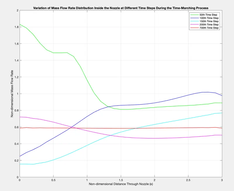
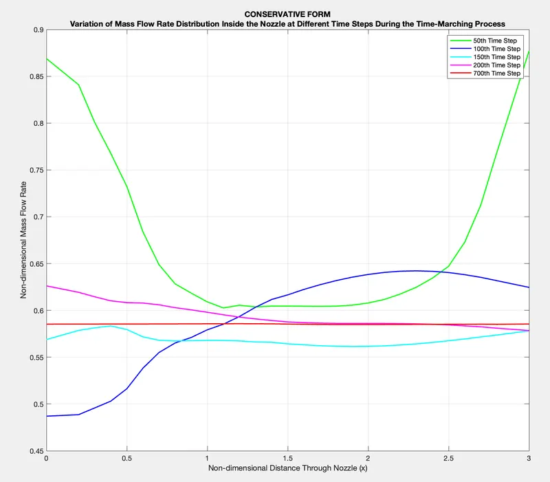
6. After all the variables have been calculated, we write a code to obtain the plot representing the variation of mass flow rate distribution inside the nozzle at different time steps during the time-marching process, in which we compare the plots at 50, 100, 150, 200 and 700 timesteps respectively.
   
   
   
   
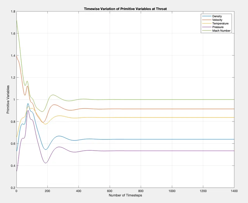
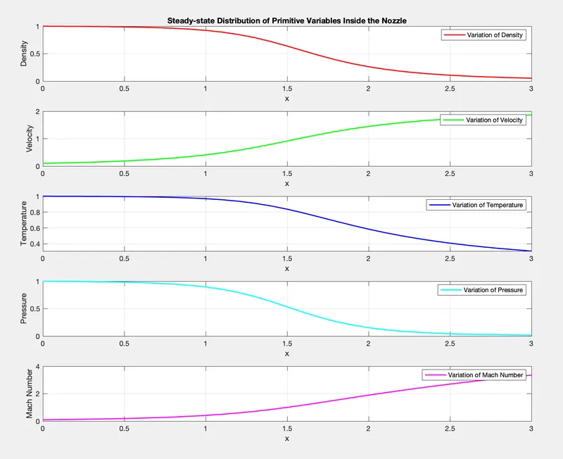
7. Similarly, we plot another graph representing timewise variation of primitive variables at the throat. Finally, we obtain another graph to represent the steady-state distribution of primitive variables inside the nozzle. We then incorporate this function code in the final program, which takes the values of the given input variables as the inputs of the function and calculates the above mentioned variables as well as the plots and thereby obtaining the required results.

Outputs for Non - Conservative Form :

By running the above program, we obtain the respective plots as follows,

1. Variation of Mass Flow Rate Distribution Inside the Nozzle at Different Time Steps During the Time-Marching Process :

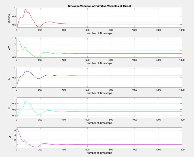
2. Timewise Variation of Primitive Variables at the Throat :

Representing all the variables in a single graph as,

3. Steady - State Distribution of Primitive Variables Inside the Nozzle :

CONSERVATIVE FORM :

The conservative form is a form of fluid flow in which the control volume does not move or is stationary with respect to the flow.

Governing Equations for Conservative Form :

The governing equations representing the continuity equation, momentum equation and the energy equation for the non – conservative form is given by,

1. Continuity Equation
   
   `(del(rho'A'))/(delt') + (del(rho'A'V'))/(delx') = 0`
   
   
   
   
2. Momentum Equation
   
   `(del(rho'A'V'))/(delt') + (del[rho'A'V'^2 + (1/gamma)P'A'])/(delx') = 1/gamma P'(delA')/(delx')`
   
   
   
   
3. Energy Equation
   
   `(del[rho'((e')/(gamma-1) + gamma/2V'^2)A'])/(delt') + (del[rho'((e')/(gamma-1) + gamma/2V'^2)V'A' + P'A'V'])/(delx') = 0`
   
   

Expressing these equations in a generic form, by defining elements of solution vector (U), flex vector (F) and the source terms (J).

Generic Forms of conservation equations are given by,

1. Solution Vectors :
   
   `U_1 = rho'A'`
   
   
   `U_2 = rho'A'V'`
   
   
   `U_3 = rho'((e')/(gamma-1) + gamma/2 V'^2)A'`
   
   
   
   
   
2. Flex Vectors :
   
   `F_1 = rho'A'V'`
   
   
   `F_2 = rho'A'V'^2 + 1/gammaP'A'`
   
   
   `F_3 = rho'((e')/(gamma-1) + gamma/2 V'^2)V'A' + P'A'V'`
   
   
   
   
   
3. Source Terms :
   
   `J_2 = 1/gammaP' (delA')/(delx')`

Using the solution vectors, flex vectors and source terms, the governing equations are written as follows,

`(delU_1)/(delt') = -(delF_1)/(delx')` `->` Continuity Equation


`(delU_2)/(delt') = -(delF_2)/(delx') + J_2` `->` Momentum Equation


`(delU_3)/(delt') = -(delF_3)/(delx')` `->` Energy Equation

MacCormack’s Method for Conservative Form :

Here, we are going to implement a finite difference MacCormack’s explicit technique to obtain the numerical solution of the governing equations.

1. Predictor Step :
   
   Initialization of flux,
   
   `F_1 = U_2`
   
   
   `F_2 = U_2^2/U_1 + (gamma-1)/gamma [U_3 - gamma/2 (U_2^2/U_1)]`
   
   
   `F_3 = gamma. (U_2 U_3)/U_1 - (gamma(gamma-1))/2 U_2^3/U_1^2`
   
   
   
   Employing predictor step in MacCormack’s method and using forward differencing scheme for spatial derivatives to calculate flex term differentials,
   
   `((delF_1)/(delx))_i^t = (F_(1_((i+1)))^t - F_(1_((i)))^t)/(dx)`
   
   
   `((delF_2)/(delx))_i^t = (F_(2_((i+1)))^t - F_(2_((i)))^t)/(dx)`
   
   
   `((delF_3)/(delx))_i^t = (F_(3_((i+1)))^t - F_(3_((i)))^t)/(dx)`
   
   
   
   Source Term :
   
   `J_(2_((i)))^t = 1/gamma.rho_iT_i((A_(i+1) - A_i)/dx)`
   
   
   Calculating time derivatives of solution vectors from space differences of `F_1`, `F_2` and `F_3`.
   
   `((delU_1)/(delt))_i^t = - ((delF_1)/(delx))_i^t`
   
   
   `((delU_2)/(delt))_i^t = - ((delF_2)/(delx))_i^t + J_(2_((i)))^t`
   
   
   `((delU_3)/(delt))_i^t = - ((delF_3)/(delx))_i^t`
   
   
   
   
   
   
   
   
   
   
   
   
   
   
2. Intermediate Solution Step :
   
   We obtain intermediate solution by using predictor values and old values of solution vector.
   
   `U_(1_((i)))^(t+Deltat) = U_(1_((i)))^(t) + ((delU_1)/(delt))_i^t . Deltat`
   
   
   `U_(2_((i)))^(t+Deltat) = U_(2_((i)))^(t) + ((delU_2)/(delt))_i^t . Deltat`
   
   
   `U_(3_((i)))^(t+Deltat) = U_(3_((i)))^(t) + ((delU_3)/(delt))_i^t . Deltat`
   
   
   
   Primitive Variables :
   
   Obtained from the updated values of `U_1`, `U_2` and `U_3`.
   
   `rho^' = U_1/A_1` ; `V^' = U_2/U_1` ; `P^' = rho^'T^'` ; `T^' = e^' = (gamma-1)(U_3/U_1 - gamma/2V^('^2))`
   
   
   
   
   
   
   
   
   
   
   
   
3. Corrector Step :
   
   Employing predictor step in MacCormack’s method and using backward differencing scheme for spatial derivatives to calculate flex term differentials,
   
   Flex Vevtors :
   
   `((delF_1)/(delx))_i^(t+Deltat) = (F_(1_((i)))^(t+Deltat) - F_(1_((i-1)))^(t+Deltat))/(dx)`
   
   
   `((delF_2)/(delx))_i^(t+Deltat) = (F_(2_((i)))^(t+Deltat) - F_(2_((i-1)))^(t+Deltat))/(dx)`
   
   
   `((delF_3)/(delx))_i^(t+Deltat) = (F_(3_((i)))^(t+Deltat) - F_(3_((i-1)))^(t+Deltat))/(dx)`
   
   
   
   Source Term :
   
   `J_(2_((i)))^(t+Deltat) = 1/gamma.rho_iT_i((A_(i) - A_(i-1))/dx)`
   
   
   
   Solution Vectors :
   
   `((delU_1)/(delt))_i^(t+Deltat) = - ((delF_1)/(delx))_i^(t+Deltat)`
   
   
   `((delU_2)/(delt))_i^(t+Deltat) = - ((delF_2)/(delx))_i^(t+Deltat) + J_(2_((i)))^(t+Deltat)`
   
   
   `((delU_3)/(delt))_i^(t+Deltat) = - ((delF_3)/(delx))_i^(t+Deltat)`
   
   
   
   
   
   
   
   
4. Final Solution Step :
   
   `((delU_1)/(delt))_("avg") = 1/2[ ((delU_1)/(delt))_i^(t) + ((delU_1)/(delt))_i^(t+Deltat)]`
   
   
   `((delU_2)/(delt))_("avg") = 1/2[ ((delU_2)/(delt))_i^(t) + ((delU_2)/(delt))_i^(t+Deltat)]`
   
   
   `((delU_3)/(delt))_("avg") = 1/2[ ((delU_3)/(delt))_i^(t) + ((delU_3)/(delt))_i^(t+Deltat)]`
   
   
   
   The final solution is obtained from calculated average derivatives and old values of solution vectors as,
   
   `U_(1_((i)))^(t+Deltat) = U_(1_((i)))^(t) + ((delU_1)/(delt))_("avg") . Deltat`
   
   
   `U_(2_((i)))^(t+Deltat) = U_(2_((i)))^(t) + ((delU_2)/(delt))_("avg") . Deltat`
   
   
   `U_(3_((i)))^(t+Deltat) = U_(3_((i)))^(t) + ((delU_3)/(delt))_("avg") . Deltat`
   
   
   
   

Initial Conditions for Conservative Form :

1. Nozzle Area :
   
   `A = 1 + 2.2(x - 1.5)^2` `"Where", 0<= x<= 3`
   
   
   
   
   
2. Initial Conditions :
   
   `"For", 0<=x'<=0.5` `{(rho' = 1.0) , (T' = 1.0):}`
   
   
   `0.5<=x'<=1.5` `{(rho' = 1.0 - 0.366(x' - 0.5)) , (T' = 1.0 - 0.167(x' - 0.5)):}`
   
   
   `1.5<=x'<=3.5` `{(rho' = 0.634 - 0.3879(x' - 1.5)) , (T' = 0.833 - 0.3507(x' - 1.5)):}`
   
   
   `V' = U_2/(rho'A') = 0.59/(rho'A')`
   
   
   
   
   
   
3. Solution Variables Initialization :
   
   `U_1 = rho'A'`
   
   
   `U_2 = rho'A'V'`
   
   
   `U_3 = rho'((e')/(gamma-1) + gamma/2 V'^2)A'`
   
   
   
   
   
   
4. Adaptive Time Method :
   
   `Deltat = "minimum"(Deltat_1^t , Deltat_2^t ...... Deltat_i^t......Deltat_N^t)`
   
   `(Deltat)_i^t = C.(Deltax)/(a_i^t + V_i^t)`
   
   

Boundary Conditions for Conservative Form :

1. Subsonic Inflow (Point 1) :
   
   `U_(1_((i=1))) = (rho'A')_(i=1) = A'_(i=1) = "fixed value"`
   
   
   `U_(2_((i=1))) = 2U_(2_((i=2))) - U_(2_((i=3)))`
   
   
   `U_3 = U_1((T')/(gamma-1) + gamma/2V'^2)`
   
   
   
   
   
2. Supersonic Outflow (Point N) :
   
   `(U_(1))_N = 2(U_(1))_(N-1) - (U_(1))_(N-2)`
   
   
   `(U_(2))_N = 2(U_(2))_(N-1) - (U_(2))_(N-2)`
   
   
   `(U_(3))_N = 2(U_(3))_(N-1) - (U_(3))_(N-2)`
   
   

Program and Explanation :

With the help of the above obtained formulas and governing equations, we write a code in MATLAB to solve for the conservative form of the equation as follows,

Conservative Function Code :

function [rho_C, V_C, T_C, P_C, mach_number_C, mass_flow_rate_C] = conservative_function(n,nt,x,dx,gamma,C)

% CALCULATING INITIAL PROFILES
% Nozzle Area and Throat Profiles
A = 1 + (2.2*(x - 1.5).^2);
throat = find(A==1);

% Initial Conditions
for i = 1:n

    if x(i)<0.5
        rho_C(i) = 1;
        T_C(i) = 1;

    elseif x(i)>=0.5 && x(i)<1.5
        rho_C(i) = 1 - (0.366*(x(i) - 0.5));
        T_C(i) = 1 - (0.167*(x(i) - 0.5));

    elseif x(i)>=1.5 && x(i)<=3.5
        rho_C(i) = 0.634 - (0.3879*(x(i) - 1.5));
        T_C(i) = 0.833 - (0.3507*(x(i) - 1.5));
    end

end

% Initial profile for Velocity
V_C = 0.59./(rho_C.*A);
P_C = rho_C.*T_C;

% Time step
%dt = min(C.*dx./(sqrt(T_C) + V_C));
dt = 0.0267;


% INITIAL SOLUTION VECTORS
U_1 = rho_C.*A;
U_2 = rho_C.*A.*V_C;
U_3 = rho_C.*((T_C./(gamma-1)) + ((gamma/2).*(V_C.^2))).*A;


% OUTER TIME-LOOP
for k = 1:nt

    % Old Variables
    U1_old = U_1;
    U2_old = U_2;
    U3_old = U_3;


    % FLUX VECTORS
    F_1 = U_2;
    F_2 = ((U_2.^2)./U_1) + (((gamma-1)/gamma) * (U_3 - ((gamma/2)*((U_2.^2)./U_1))));
    F_3 = (gamma.*((U_2.*U_3)./U_1)) - ((gamma.*(gamma-1))/2).*((U_2.^3)./(U_1.^2));


    % MACCORMACK'S METHOD
    % PREDICTOR STEP
    % For inner nodes
    for j = 2:n-1

        % Source Term
        J_2(j) = (1/gamma)*rho_C(j)*T_C(j)* ((A(j+1) - A(j))/dx);


        % DISCRETIZED GOVERNING EQUATIONS
        % Continuity Equation
        dU1_dt_p(j) = - ((F_1(j+1) - F_1(j))./dx);

        % Momentum Equation
        dU2_dt_p(j) = - ((F_2(j+1) - F_2(j))./dx) + J_2(j);

        % Energy Equation
        dU3_dt_p(j) = - ((F_3(j+1) - F_3(j))./dx);


        % INTERMEDIATE SOLUTION STEP
        % Updating Values
        U_1(j) = U_1(j) + (dU1_dt_p(j)*dt);
        U_2(j) = U_2(j) + (dU2_dt_p(j)*dt);
        U_3(j) = U_3(j) + (dU3_dt_p(j)*dt);

    end


    % Updating Flex Vectors
    F_1 = U_2;
    F_2 = ((U_2.^2)./U_1) + (((gamma-1)./gamma) * (U_3 - ((gamma/2)*((U_2.^2)./U_1))));
    F_3 = (gamma.*((U_2.*U_3)./U_1)) - ((gamma.*(gamma-1))/2).*((U_2.^3)./(U_1.^2));


    % CORRECTOR STEP
    % For inner nodes
    for j = 2:n-1

        % Updating Source Term
        J_2(j) = (1/gamma)*rho_C(j)*T_C(j)* ((A(j) - A(j-1))/dx);


        % DISCRETIZED GOVERNING EQUATIONS
        % Continuity Equation
        dU1_dt_c(j) = - ((F_1(j) - F_1(j-1))/dx);

        % Momentum Equation
        dU2_dt_c(j) = - ((F_2(j) - F_2(j-1))/dx) + J_2(j);

        % Energy Equation
        dU3_dt_c(j) = - ((F_3(j) - F_3(j-1))/dx);

    end


    % Computing Average Time Derivative
    dU1_dt = 0.5*(dU1_dt_p + dU1_dt_c);
    dU2_dt = 0.5*(dU2_dt_p + dU2_dt_c);
    dU3_dt = 0.5*(dU3_dt_p + dU3_dt_c);


    % Final Solution Update
    for i = 2:n-1

        U_1(i) = U1_old(i) + (dU1_dt(i)*dt);
        U_2(i) = U2_old(i) + (dU2_dt(i)*dt);
        U_3(i) = U3_old(i) + (dU3_dt(i)*dt);

    end

    % BOUNDARY CONDITIONS
    % Subsonic Inflow (point 1)
    U_1(1) = rho_C(1) * A(1);
    U_2(1) = (2*U_2(2)) - U_2(3);
    U_3(1) = U_1(1) * ((T_C(1)/(gamma-1)) + ((gamma/2)*(V_C(1).^2)));
    V_C(1) = U_2(1)/U_1(1);

    % Supersonic Outflow (point n)
    U_1(n) = (2*U_1(n-1)) - U_1(n-2);
    U_2(n) = (2*U_2(n-1)) - U_2(n-2);
    U_3(n) = (2*U_3(n-1)) - U_3(n-2);



    % PRIMITIVE VARIABLES
    % Density
    rho_C = U_1./A;

    % Velocity
    V_C = U_2./U_1;

    % Temperature
    T_C = (gamma-1) .* ((U_3./U_1) - ((gamma/2).*(V_C.^2)));


    % OUTPUT VARIABLES
    % Mass Flow Rate, m = rho*A*V
    mass_flow_rate_C = rho_C.*A.*V_C;

    % Pressure
    P_C = rho_C.*T_C;

    % Mach Number
    mach_number_C = V_C./(T_C.^0.5);


    % Calculating Variables at Throat Section
    rho_throat_C(k) = rho_C(throat);
    V_throat_C(k) = V_C(throat);
    T_throat_C(k) = T_C(throat);
    mass_flow_rate_throat_C(k) = mass_flow_rate_C(throat);
    P_throat_C(k) = P_C(throat);
    mach_number_throat_C(k) = mach_number_C(throat);


    % PLOTTING
    % Variation of Mass flow rate distribution inside the nozzle at different time steps during the time-marching process
    figure(4)

    if k == 50
        plot(x,mass_flow_rate_C,'color','g','LineWidth',1.5)
        hold on

    elseif k == 100
        plot(x,mass_flow_rate_C,'color','b','LineWidth',1.5)
        hold on

    elseif k == 150
        plot(x,mass_flow_rate_C,'color','c','LineWidth',1.5)
        hold on

    elseif k == 200
        plot(x,mass_flow_rate_C,'color','m','LineWidth',1.5)
        hold on

    elseif k == 700
        plot(x,mass_flow_rate_C,'color','r','LineWidth',1.5)
        hold on
        title({'CONSERVATIVE FORM','Variation of Mass Flow Rate Distribution Inside the Nozzle at Different Time Steps During the Time-Marching Process'})
        xlabel('Non-dimensional Distance Through Nozzle (x)')
        ylabel('Non-dimensional Mass Flow Rate')
        legend('50th Time Step','100th Time Step','150th Time Step','200th Time Step','700th Time Step')
        grid on
    end
end


% PLOTTING
% Timewise Variation of Primitive Variables at Throat
figure(5)

% Density
subplot(5,1,1)
plot(rho_throat_C,'LineWidth',1,'Color','r')
title('Timewise Variation of Primitive Variables at Throat')
xlabel('Number of Timesteps')
ylabel('rho/rho_o')
grid on

% Velocity
subplot(5,1,2)
plot(V_throat_C,'LineWidth',1,'Color','g')
xlabel('Number of Timesteps')
ylabel('V/V_o')
grid on

% Temperature
subplot(5,1,3)
plot(T_throat_C,'LineWidth',1,'Color','b')
xlabel('Number of Timesteps')
ylabel('T/T_o')
grid on

% Pressure
subplot(5,1,4)
plot(P_throat_C,'LineWidth',1,'Color','c')
xlabel('Number of Timesteps')
ylabel('P/P_o')
grid on

% Mach Number
subplot(5,1,5)
plot(mach_number_throat_C,'LineWidth',1,'Color','m')
xlabel('Number of Timesteps')
ylabel('M')
grid on





% Steady-state distribution of primitive variables inside the nozzle
figure(6)

% Density
subplot(5,1,1)
plot(x,rho_C,'Color','r','LineWidth',1.5)
xlabel('x')
ylabel('Density')
legend('Variation of Density')
title('Steady-state Distribution of Primitive Variables Inside the Nozzle')
grid on

% Velocity
subplot(5,1,2)
plot(x,V_C,'Color','g','LineWidth',1.5)
xlabel('x')
ylabel('Velocity')
legend('Variation of Velocity')
grid on

% Temperature
subplot(5,1,3)
plot(x,T_C,'Color','b','LineWidth',1.5)
xlabel('x')
ylabel('Temperature')
legend('Variation of Temperature')
grid on

% Pressure
subplot(5,1,4)
plot(x,P_C,'Color','c','LineWidth',1.5)
xlabel('x')
ylabel('Pressure')
legend('Variation of Pressure')
grid on

% Mach Number
subplot(5,1,5)
plot(x,mach_number_C,'Color','m','LineWidth',1.5)
xlabel('x')
ylabel('Mach Number')
legend('Variation of Mach Number')
grid on

end

Final Program for Conservative Form :

% 1-D QUASI SUBSONIC - SUPERSONIC NOZZLE FLOW SIMULATION
clear all
close all 
clc


% INPUTS
% Length of nozzle
L = 3; 

% Number of grid points
n = 31;

% Number of Timesteps
nt = 1400; 

% Defining the mesh
x = linspace(0,L,n);

% Grid Spacing
dx = x(2) - x(1);

% Ratio of Specific Heats
gamma = 1.4;

% Courant Number
C = 0.5; 


% DEFINING THE FUNCTIONS
% NON-CONSERVATIVE FORM FUNCTION
tic
[rho_NC, V_NC, T_NC, P_NC, mach_number_NC, mass_flow_rate_NC] = non_conservative_function(n,nt,x,dx,gamma,C)
non_conservative_time = toc

% CONSERVATIVE FORM FUNCTION
tic
[rho_C, V_C, T_C, P_C, mach_number_C, mass_flow_rate_C] = conservative_function(n,nt,x,dx,gamma,C)
conservative_time = toc


% PLOTTING
% Comparison of Normalized mass flow rate distributions of both forms
figure(7)
plot(x,mass_flow_rate_NC,'LineWidth',1.5)
hold on
plot(x,mass_flow_rate_C,'LineWidth',1.5)
title('Comparison of Normalized Mass Flow Rate Distributions of both forms')
xlabel('x')
ylabel('Mass Flow Rate')
legend('Non-Conservative Form','Conservative Form')
grid on

Code Explanation :

1. We begin the program by defining a function for the conservative form, which takes the inputs provided and outputs the values of the respective terms we are going to incorporate in the function along the way.
   
   
   
2. In the next step, we employ the various initial conditions to initialize the conditions for `rho` and `T` for the range of values of “`x`”, from the formulae we have already mentioned above.
   We also calculate the initial profiles of density, temperature, velocity and area of the nozzle with the help of the conditions which we have previously defined. We also calculate the throat of the nozzle by finding the position of the nozzle where the area is the least (1).
   
   
   
3. In the next step, we calculate the value of the time-step (`dt`) and we also define the initial solution vectors `U_1`, `U_2` and `U_3`.
   
   
   
4. Next, we define an outer time loop for the range of 1 to the number of timesteps (`nt`). We assign the values of the initial solution vectors `U_1`, `U_2` and `U_3` to three new arrays namely `U_(1_(old))`, `U_(2_(old))` and `U_(3_(old))` respectively. We also define the values of the flux vectors `F_1`, `F_2` and `F_3` with the help of the formulae mentioned above.
   
   
   
5. In the next step, we are going to implement a finite difference MacCormack’s explicit technique to obtain the numerical solution of the governing equations.
   
   In the Predictor Step, we are using forward differencing scheme for the flex vector terms, to discretize the continuity, momentum and energy governing equations. We are also going to calculate the value of the source term (`J_2`). Further, we are going to calculate solution variant for which we obtain an intermediate solution in which we are finding the solution vectors at time " `t + Deltat` " from solution gradients and old solution vector values.
   
   Before moving to the corrector step, we first update the new values of the flux vectors. In the Corrector Step, we first obtain a corrected value of time derivative at time “ `t+Deltat` ”. These corrected values are obtained by substituting values of flux vectors `F_1`, `F_2` and `F_3` into R.H.S of equation and replacing spatial derivative with the backward differencing scheme.
   
   In the final solution step, we are going to calculate average value of time derivatives of solution vectors, which are obtained from the arithmetic mean of predictor and corrector step. This allows us to obtain the final values of `U_1`, `U_2` and `U_3` at time `t+Deltat`.
   
   
   
   
   
6. Before moving on to the next step, we define the inlet and outlet boundary conditions for the nozzle and thereby, we calculate the mass flow rate, pressure and mach number for the same. Similarly, we calculate the variables at the throat section of the nozzle.
   
   
   
   
7. After all the variables have been calculated, we write a code to obtain the plot representing the variation of mass flow rate distribution inside the nozzle at different time steps during the time-marching process, in which we compare the plots at 50, 100, 150, 200 and 700 timesteps respectively for the conservation form.
   
   
   
8. Similarly, we plot another graph representing timewise variation of primitive variables at the throat.
   
   
   
9. Finally, we obtain another graph to represent the steady-state distribution of primitive variables inside the nozzle. We then incorporate this function code in the final program, which takes the values of the given input variables as the inputs of the function and calculates the above mentioned variables as well as the plots and thereby obtaining the required results.
   
   
   
   
10. Finally, we obtain a plot to represent the comparison of normalized mass flow rate distributions of both the Conservative and Non-Conservative forms.

Outputs for Conservative Form :

By running the above program, we obtain the respective plots as follows,

1. Variation of Mass Flow Rate Distribution Inside the Nozzle at Different Time Steps During the Time-Marching Process :

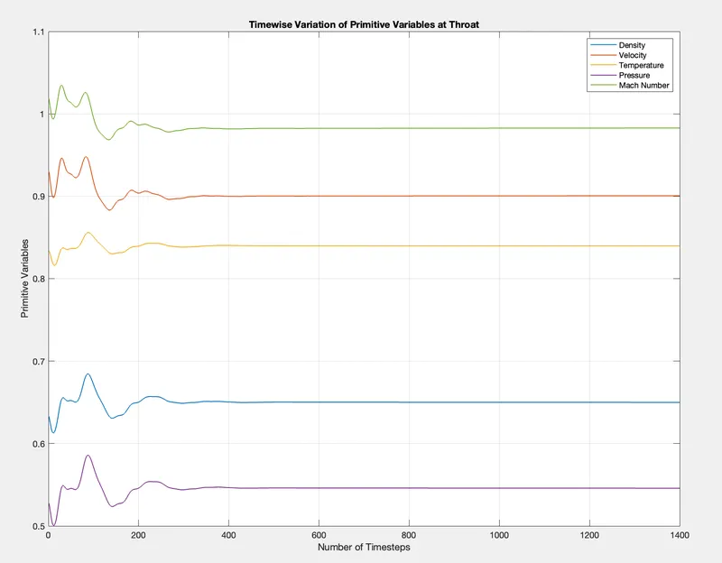
2. Timewise Variation of Primitive Variables at the Throat :

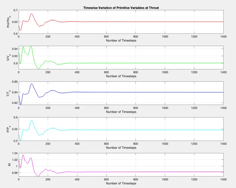
Representing all the variables in a single graph as,

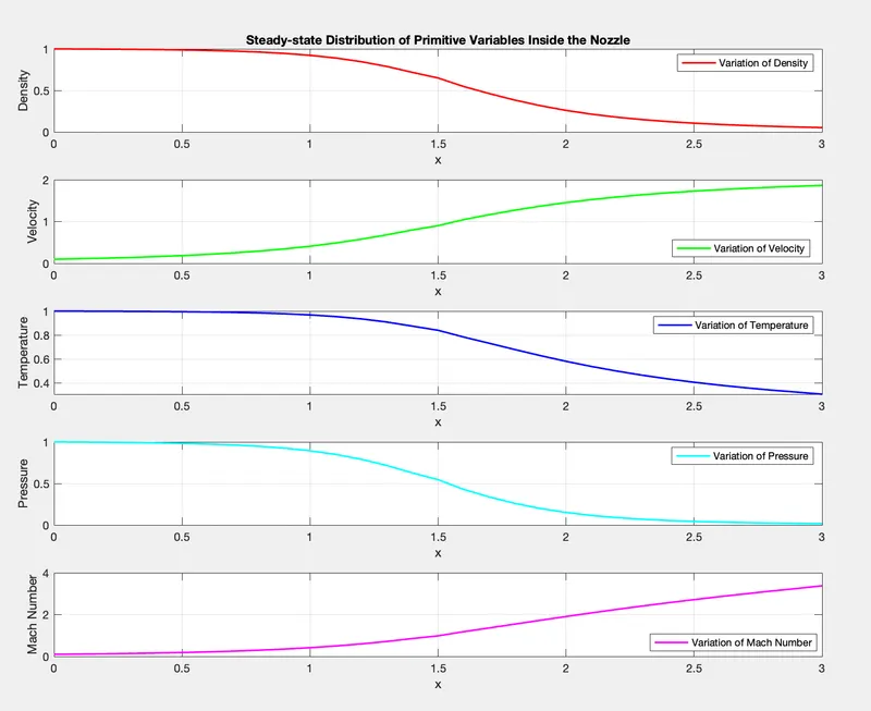
3. Steady - State Distribution of Primitive Variables Inside the Nozzle :

GRID INDEPENDENCE TEST :

The grid independence test is a process used to find the optimal grid condition that has the smallest number of grids without generating a difference in the numerical results based on the evaluation of various grid conditions.

Here, we are going to conduct a grid independence test on the 1-D subsonic – supersonic nozzle flow problem by increasing the number of grid points from 31 to 61. We obtain the primitive data values for the conservative and non-conservative forms as shown below.

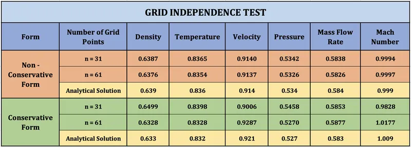
From the above data, we can observe that, even with the increase in the number of grid points, there is no effect on the primitive variable values for both the conservative and non- conservative forms. We can also observe that, with the increase in the number of grid points, the numerical solution values are much closer to the analytical or real solution of the equation, when compared to that of the lesser number of grid points.

Therefore, from the above data and observations, we can clearly say that the 1-D subsonic – supersonic problem is grid independent.

CONCLUSION :

• The MATLAB code to simulate the steady-state distribution for the flow-field variables of the Quasi 1-D Subsonic – Supersonic Nozzle Flow has been written and executed for both the conservative and non-conservative forms, using the MacCormack’s Technique.
  
  
  
• From the respective plots obtained for both the conservative and non-conservative forms, we can observe that the mass flow distribution is more consistent for the conservative form and thereby it does a better job at conserving mass, when compared to the non-conservative form.
  
  
  
• And also, the time required to run the simulation is marginally higher for the conservative form as compared to the non-conservative form because the calculation time required to decode the primitive variables to the flux vector in the conservative form is more.
  
  
• Consequently, we can also observe that, an increase in the number of grid points leads to a higher accuracy or closeness of the numerical solution to the analytical or real solution. Thereby, the non-conservative form gives accurate results with respect to the primitive variables whereas the conservative form does a better job at providing accurate results for the flux variables.
  
  
  
• Finally, from the primitive variable data table represented above, we can conclude that both the conservative and non-conservative forms of the equation are grid independent. Meaning, a change in the number of grid points does not affect the numerical solution.