Genetic Algorithm

OBJECTIVE :

• Write a code in MATLAB to optimize the stalagmite function and find the global maxima of the function.
• Explain the concepts of genetic algorithm and also explain the syntax of ga in MATLAB.
• Make sure that the code gives the same output, even if it is made to run several times.
• Plot graph for all 3 studies and for F maximum vs number of iterations.

INTRODUCTION :

A genetic algorithm is a search based optimization technique that is inspired by Charles Darwin’s theory of natural evolution. This algorithm reflects the process of natural selection where the fittest individuals are selected for reproduction in order to produce offspring of the next generation.

In other words, a genetic algorithm is an optimization technique, which tries to find out such values of input so that we get the best output value (optimal or near optimal results).

The working of a genetic algorithm is as shown below.

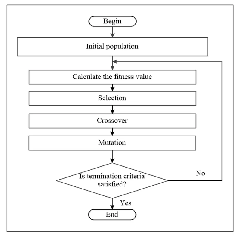
The evolution usually starts from a population of randomly generated individuals, and is an iterative process, with the population in each iteration called a generation. In each generation, the fitness of every individual in the population is evaluated. The fitness is usually the value of the objective function in the optimization problem being solved. The more fit individuals are stochastically selected from the current population, and each individual's genome is modified (recombined and possibly randomly mutated) to form a new generation. The new generation of candidate solutions is then used in the next iteration of the algorithm. Commonly, the algorithm terminates when either a maximum number of generations has been produced, or a satisfactory fitness level has been reached for the population.

1. Initial Population ( Initialization) :

The process begins with a set of individuals which is called a Population. An individual is characterized by a set of parameters (variables) known as Genes. Genes are joined into a string to form a Chromosome (solution).

The chromosomes are binary strings (string of 1s and 0s). We say that we encode the genes in a chromosome.

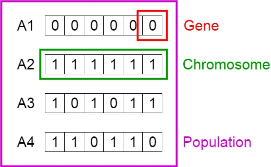
The population size depends on the nature of the problem, but typically contains several hundreds or thousands of possible solutions. Often, the initial population is generated randomly, allowing the entire range of possible solutions.

2. Fitness Function :

The fitness function determines how fit an individual is (the ability of an individual to compete with other individuals). It gives a fitness score to each individual. The probability that an individual will be selected for reproduction is based on its fitness score.

3. Selection :

The idea of selection phase is to select the fittest individuals and let them pass their genes to the next generation. Two pairs of individuals (parents) are selected based on their fitness scores. Individuals with high fitness have more chance to be selected for reproduction.

General thought is that we should select the fit chromosomes and allow them to produce off-springs. But that would lead to chromosomes that are more close to one another in a few next generations, and therefore less diversity. Therefore, we generally use Roulette Wheel Selection method.

Based on the fitness values, we create the roulette wheel as follows :

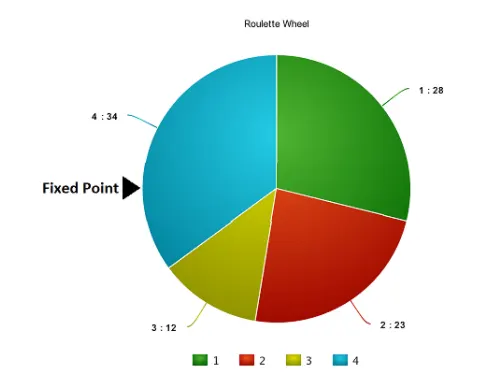
So, now this wheel is rotated and the region of wheel which comes in front of the fixed point is chosen as the parent. For the second parent, the same process is repeated.

Sometimes we mark two fixed point as shown in the figure below.

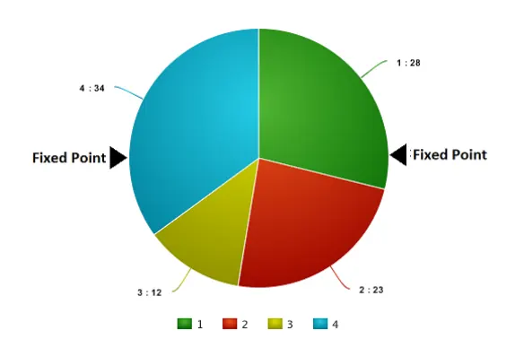
So, in this method we can get both our parents in one go. This method is known as Stochastic Universal Selection method.

4. Crossover :

Crossover is the most significant phase in a genetic algorithm. For each pair of parents to be mated, a crossover point is chosen at random from within the genes. Offspring are created by exchanging the genes of parents among themselves.

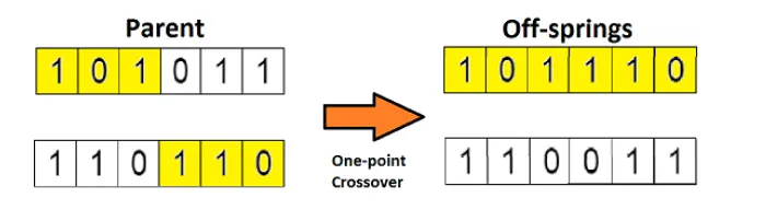
This is the most basic form of crossover, known as one point crossover. Here we select a random crossover point and the tails of both the chromosomes are swapped to produce a new off-springs.

If you take two crossover points, then it will called as multi point crossover which is as shown below.

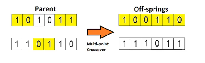
The new offsprings are added to the population.

5. Mutation :

In certain new offsprings formed, some of their genes can be subjected to a change, with a low random probability. This implies that some of the bits in the bit string can be flipped. This process is known as mutation, which may be defined as a random tweak in the chromosome, which also promotes the idea of diversity in the population.

A simple method of mutation is shown in the image below.

6. Termination :

The algorithm terminates if the population has converged (does not produce offspring which are significantly different from the previous generation). Then it is said that the genetic algorithm has provided a set of solutions to our problem.

Basically there are different termination conditions, which are listed below:

1. There is no improvement in the population for over x iterations.
2. We have already predefined an absolute number of generation for our algorithm.
3. When our fitness function has reached a predefined value.

GENETIC ALGORITHM SYNTAX :

The general syntax of a Genetic Algorithm ( ga ) function is given by,

[x,fval,exitflag,output,population,scores] = ga(fun,nvars,A,b,Aeq,beq,lb,ub,nonlcon,intcon,options)

Where,

x = local minimum for structure defined in problem

fval = the value of fitness function at ‘x’

exitflag = an integer identifying the reason the algorithm terminated

output = a structure that contains output from each generation and other information about the performance of the algorithm

population = returns a matrix population, whose rows are the final population

scores = the scores of the final population

fun = objective function

nvars = number of design variables of fun

A , b = linear inequalities

Aeq , beq = linear equalities

lb = lower bounds on the design variables

ub = upper bounds on the design variables

nonlcon = subjects the minimization to the constraints defined in nonlcon

intcon = requires that the variables listed in intcon take integer values

options = minimizes with the default optimization parameters replaced by values in options.

GOVERNING EQUATIONS :

The general equations to create a stalagmite function are given by,

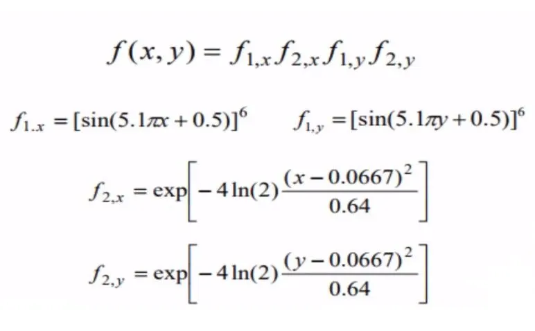
Let us consider, `f_(1x) = [sin(5.1pix + 0.5)]^6` as equation - 1

And `f_(1y) = [sin(5.1piy + 0.5)]^6` as equation - 2

In the second set of equations, let us consider

`A = (x - 0.0667)^2/0.64`

Therefore, `f_(2x) = exp[-4ln(2)*A]` equation - 3

Similarly, `B = (y - 0.0667)^2/0.64`

Therefore, `f_(2y) = exp[-4ln(2)*B]` equation - 4

DETAILED PROCEDURE AND EXPLANATION OF STALAGMITE MODEL PROGRAMMING :

Step – 1 :

The first and foremost step in creating a program to obtain the model of a stalagmite is to define our searchspace by creating 1 dimensional arrays x and y, containing 150 elements between 0 and 0.6.

Code :

% defining the searchspace
x = linspace(0,0.6,150);
y = linspace(0,0.6,150);

After the searchspace has been defined, we then create a 2 dimensional array of x and y by using the meshgrid function. The meshgrid command returns 2-D grid coordinates based on coordinates contained in vectors x and y.

Code :

% creating a 2D mesh
[xx yy] = meshgrid(x,y);

Step – 2 :

Before heading further, we first need to create a stalagmite function based on the equations. With reference to the equations we have already defined above, we get the function code as follows.

Considering the equations – 1 , 2 , 3 and 4, we define the stalagmite function as follows:

Code :

function [f] = stalagmite(input_vector)

x = input_vector(1);
y = input_vector(2);

% first set of equations
f1_x = (sin(5.1*pi*x + 0.5)).^6
f1_y = (sin(5.1*pi*y + 0.5)).^6

% second set of equations
A = ((x-0.0667).^2)/(0.64)
f2_x = exp(-4.*log(2)*A)

B = ((y-0.0667).^2)/(0.64)
f2_y = exp(-4.*log(2)*B)

f = -(f1_x.*f2_x.*f1_y.*f2_y)
end

Wherein, the equations for f1_x , f1_y , f2_x and f2_y are defined as shown in the governing equations section. That is, equations 1 , 2 , 3 and 4.

The above stalagmite function is then incorporated into the main program, as a function.

Step – 3 :

After defining the stalagmite function, the next step is incorporating it in the ‘for loop’, to create the dataset. A number of iterations of the for loop is run till the optimal solution is reached or the criteria is satisfied.

Code :

% for loop function
for i = 1:length(xx);
    for j = 1:length(yy);

        input_vector(1) = xx(i,j)
        input_vector(2) = yy(i,j)
        f(i,j) = stalagmite(input_vector);
    end
end

Finally, with reference to the above data, a surface graph is plotted to show the stalagmite model. The "shading interp" command is used to remove grid lines from the plot and give a smooth surface look.

Final code :

% stalagmite model
clear all
close all
clc

% providing searchspace
x = linspace(0,0.6,150);
y = linspace(0,0.6,150);

% creating 2D mesh
[xx yy] = meshgrid(x,y);

% number of iterations
num_cases = 50

% for loop function
for i = 1:length(xx);
    for j = 1:length(yy);

        input_vector(1) = xx(i,j)
        input_vector(2) = yy(i,j)
        f(i,j) = stalagmite(input_vector);
    end
end

% plotting
figure(1)
surfc(xx,yy,-f)
shading interp

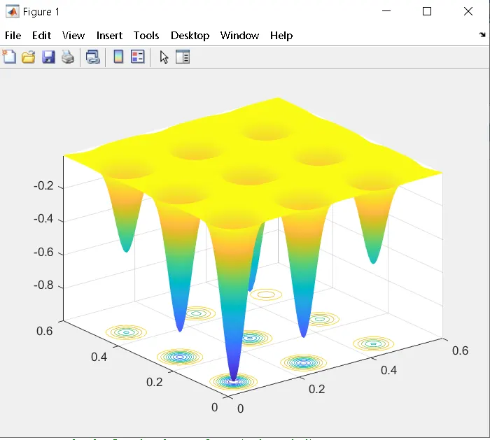
OUTPUT PLOT :

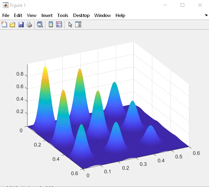
The above graph represents the output stalagmite model of the program.

STATISTICAL CASE STUDIES :

Case 1 : Statistical Behaviour of GA subjected to no Bounds (Unbounded)

In this case study, we consider the ga subjected to no bounds.

for loop :

• First, we call the function using the ‘for loop’ and by passing the variable number as 2, we obtain optimum values of x (xopt) and y (yopt).
  
  
• We use the tic and toc commands to evaluate the elapsed time to run the code, in seconds. The tic function records the current time and the toc function uses the recorded value to calculate the elapsed time.

Plotting :

• We use subplots to create multiple plots inside the same figure window.
  
  
• We use the plot3 function over the 50 studies to visualise how the algorithm is functioning and to obtain a 3D visualization of the points.
  
  
• We plot a second subplot of the optimum function value the ga is predicting (fopt), as a function of the iterations.
  
  
• As ga always predicts the minimum value of the function, we use a negative sign ‘-‘ to obtain an inverted image of the plot so we can calculate the maximum value.

Code :

% case 1 - Statistical Behaviour of GA (unbounded)
tic
for i = 1:num_cases
    [inputs,fopt(i)] = ga(@stalagmite,2)
    xopt(i) = inputs(1)
    yopt(i) = inputs(2)
end

study1_time = toc

% plotting case study 1
figure(2)
subplot(2,1,1)
surfc(xx,yy,-f)
shading interp
hold on
plot3(xopt,yopt,-fopt,'Marker','o','MarkerSize',5,'MarkerFaceColor','r')
subplot(2,1,2)
plot(-fopt)
title('Unbounded Inputs')
xlabel('Iterations')
ylabel('Function Maximum Value')

Output :

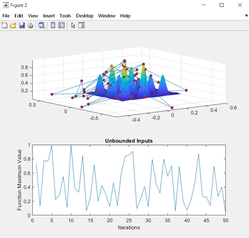
From the results, we can observe that the results are pretty inaccurate and do a bad job at optimising the function as, the points are scattered all over the place.

Case 2 : Statistical Behaviour of GA subjected to Upper and Lower Bounds (Bounded)

• In the first step, we set the upper and lower bounds for the variables, in the ga syntax between 0 and 1. For the other undefined variables in the syntax, we enter ‘ [ ] ‘.
  
  
• Similar to the first case, we run the 'for loop' to obtain the optimum values of x (xopt), y (yopt) and fopt. We also, record the elapsed time by using the tic and toc command.
  
  
• We then obtain the plots and subplots, similarly representing the stalagmite plot, the algorithm functioning over the 50 iterations and a subplot of optimum function value (fopt), over a much narrower range as compared to case 1.

Code :

% case 2 - Statistical Behaviour of GA subjected to Upper and Lower Bounds
tic
for j = 1:num_cases
    [inputs,fopt(j)] = ga(@stalagmite,2,[],[],[],[],[0;0],[1;1])
    xopt(j) = inputs(1)
    yopt(j) = inputs(2)
end

study2_time = toc

% plotting case study 2
figure(3)
subplot(2,1,1)
surfc(xx,yy,-f)
shading interp
hold on
plot3(xopt,yopt,-fopt,'Marker','o','MarkerSize',5,'MarkerFaceColor','r')
subplot(2,1,2)
plot(-fopt)
title('Bounded Inputs')
xlabel('Iterations')
ylabel('Function Maximum Value')

Output :

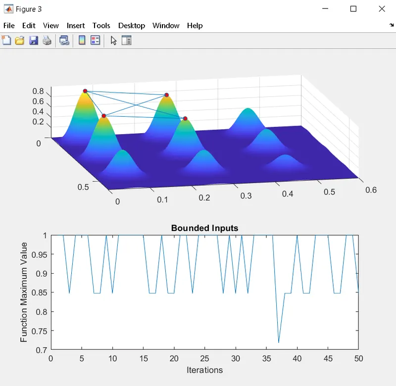
From the above output, we can determine that the maximum point or global maxima lies between the 4 peaks of the stalagmite function. And also, the range of the function maximum value has reduced to the range of 0.7 - 1, which was previously in the range 0 - 1. The above output is still not exactly accurate and thereby, moving on to the third case.

Case 3 : Statistical Behaviour of GA subjected to Increase in Population Size

• In this case study, in addition to specifying the bounds, we are going to increase the population size.
  
  
• With reference to case 2, if the population size is too less, the algorithm calculates the local maxima instead of the global maxima. Thereby, we overcome this issue by increasing the population size.
  
  
• We are going to use the ‘optimoptions’ function to define the new population size of the function as 300.
  
  
• As a result of the increase in population size, the program is going to take longer to produce the outputs.

Code :

% case 3 - Increasing the Population Size
options = optimoptions("ga",'PopulationSize',300)

tic
for k = 1:num_cases
    [inputs,fopt(k)] = ga(@stalagmite,2,[],[],[],[],[0;0],[1;1],[],[],options)
    xopt(k) = inputs(1)
    yopt(k) = inputs(2)
end

study3_time = toc

% plotting case study 2
figure(4)
subplot(2,1,1)
surfc(xx,yy,-f)
shading interp
hold on
plot3(xopt,yopt,-fopt,'Marker','o','MarkerSize',5,'MarkerFaceColor','r')
subplot(2,1,2)
plot(-fopt)
title('Increased Population')
xlabel('Iterations')
ylabel('Function Maximum Value')

Output :

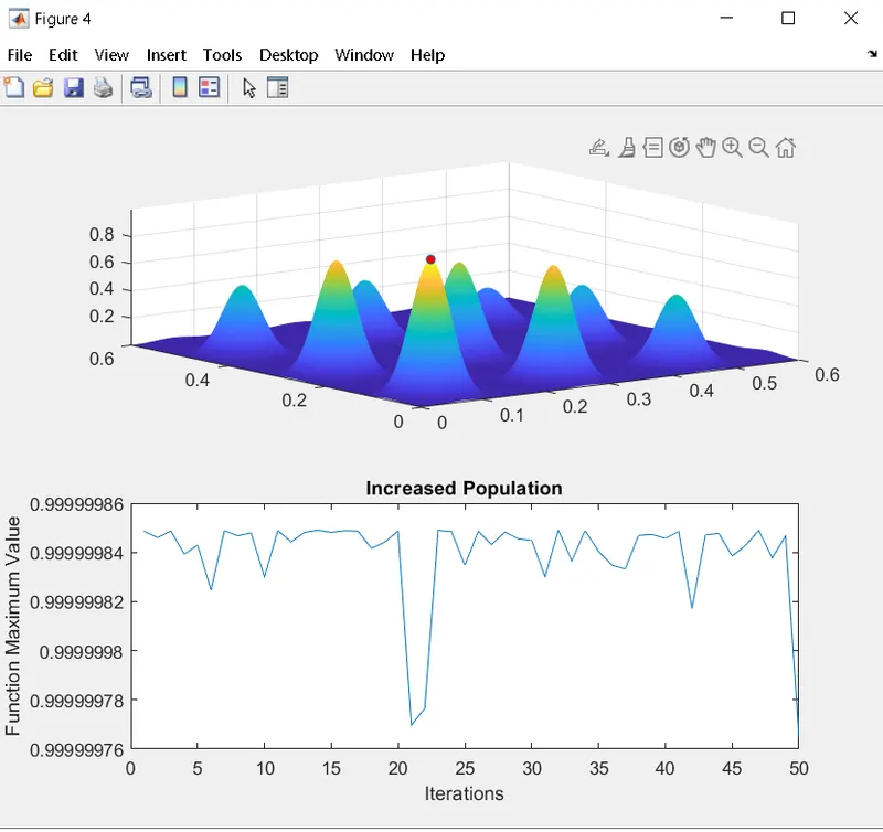
From the above output graph, we can conclude that the results are the most accurate, with the range precisely narrowed down and thereby, we obtain the global maxima value of the stalagmite function and the stalagmite function is optimized.

FINAL PROGRAM CODE TO OPTIMIZE STALAGMITE FUNCTION :

% stalagmite model
clear all
close all
clc

% providing searchspace
x = linspace(0,0.6,150);
y = linspace(0,0.6,150);

% creating 2D mesh
[xx yy] = meshgrid(x,y);

% number of iterations
num_cases = 50

% for loop function
for i = 1:length(xx);
    for j = 1:length(yy);

        input_vector(1) = xx(i,j)
        input_vector(2) = yy(i,j)
        f(i,j) = stalagmite(input_vector);
    end
end

% plotting
figure(1)
surfc(xx,yy,-f)
shading interp


% case studies
% case 1 - Statistical Behaviour of GA (unbounded)
tic
for i = 1:num_cases
    [inputs,fopt(i)] = ga(@stalagmite,2)
    xopt(i) = inputs(1)
    yopt(i) = inputs(2)
end

study1_time = toc

% plotting case study 1
figure(2)
subplot(2,1,1)
surfc(xx,yy,-f)
shading interp
hold on
plot3(xopt,yopt,-fopt,'Marker','o','MarkerSize',5,'MarkerFaceColor','r')
subplot(2,1,2)
plot(-fopt)
title('Unbounded Inputs')
xlabel('Iterations')
ylabel('Function Maximum Value')


% case 2 - Statistical Behaviour of GA subjected to Upper and Lower Bounds
tic
for j = 1:num_cases
    [inputs,fopt(j)] = ga(@stalagmite,2,[],[],[],[],[0;0],[1;1])
    xopt(j) = inputs(1)
    yopt(j) = inputs(2)
end

study2_time = toc

% plotting case study 2
figure(3)
subplot(2,1,1)
surfc(xx,yy,-f)
shading interp
hold on
plot3(xopt,yopt,-fopt,'Marker','o','MarkerSize',5,'MarkerFaceColor','r')
subplot(2,1,2)
plot(-fopt)
title('Bounded Inputs')
xlabel('Iterations')
ylabel('Function Maximum Value')


% case 3 - Increasing the Population Size
options = optimoptions("ga",'PopulationSize',300)

tic
for k = 1:num_cases
    [inputs,fopt(k)] = ga(@stalagmite,2,[],[],[],[],[0;0],[1;1],[],[],options)
    xopt(k) = inputs(1)
    yopt(k) = inputs(2)
end

study3_time = toc

% plotting case study 2
figure(4)
subplot(2,1,1)
surfc(xx,yy,-f)
shading interp
hold on
plot3(xopt,yopt,-fopt,'Marker','o','MarkerSize',5,'MarkerFaceColor','r')
subplot(2,1,2)
plot(-fopt)
title('Increased Population')
xlabel('Iterations')
ylabel('Function Maximum Value')

PROBLEMS ENCOUNTERED :

1. While defining the stalagmite function, i forgot to incorporate the minus sign in the function, as a result of which, i obtained an inverted graph of the outputs.

Supposed to be :

Mistake :

Error Output :

CONCLUSIONS :

1. The code to optimize the stalagmite function has been written and the global maxima of the function has been obtained.
   
   
2. The Genetic Algorithm has been explained along with its syntax and individual functions.
   
   
3. All three case studies signifying the statistical behaviour of the GE function when it is unbounded, bounded and when it is subjected to an increase in population, have been discussed and the output graphs have been plotted.
   
   
4. It is observed that the function has been fully optimized when subjected to constraints and with an increased population, thereby reducing the range of the function maximum value for the total number of iterations and therefore the global maxima is obtained.

REFERENCES :

https://en.wikipedia.org/wiki/Genetic_algorithm

https://towardsdatascience.com/introduction-to-genetic-algorithms-including-example-code-e396e98d8bf3

https://www.sciencedirect.com/topics/engineering/genetic-algorithm

https://in.mathworks.com/help/gads/ga.html#d123e44712