Week 5 - Rayleigh Taylor Instability
AIM :
To carry out Rayleigh Taylor Instability Analysis for a multi-phase fluid.
OBJECTIVES :
- In your own words, explain what are some practical CFD models that have been based on the mathematical analysis of Rayleigh Taylor waves and how these mathematical models have been adapted for CFD calculations.
- Perform the Rayleigh Taylor instability simulation for 2 different mesh sizes with the base mesh being 5 mm. Compare the results by showing the animations. Observe the differences in the animation and explain the effect of mesh size on simulation.
- Explain why a steady-state approach might not be suitable for these types of simulation.
- Run one more simulation with water and user-defined material(density = 400 kg/m3, viscosity = 0.001 kg/m-s) for refined mesh.
- Define the Atwood Number. Find out the Atwood number for both the cases and explain how the variation in Atwood number in the above two cases affects the behaviour of the instability.
INTRODUCTION :
The Rayleigh–Taylor instability, or RT instability, is an instability of an interface between two fluids of different densities which occurs when the lighter fluid is pushing the heavier fluid. It is a dynamic process whereby the two fluids seek to reduce their combined potential energy.
Examples include the behaviour of water suspended above oil in the gravity of Earth, mushroom clouds like those from volcanic eruptions and atmospheric nuclear explosions. This situation has engineering implications in several industries such as in die casting, where liquid metal is injected in a cavity filled with air.
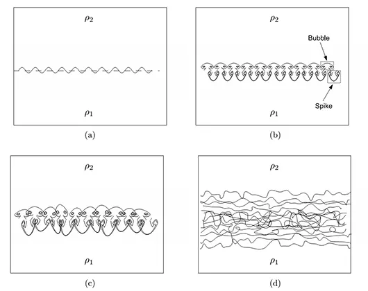
This figure represents the evolution of the Rayleigh–Taylor instability from small wavelength perturbations at the interface (a) which grow into mushroom shaped spikes (fluid structures of heavy into light fluid) and bubbles (fluid structures of light into heavy fluid) (b) and these fluid structures interact due to bubble merging and competition (c) eventually developing into a mixing region (d). Here `rho_2` represents the heavy fluid and `rho_1` represents the light fluid. Gravity is acting downward and the system is RT unstable.
What are some practical CFD models that have been based on the mathematical analysis of Rayleigh Taylor waves?
The free surface flows are successfully modelled with one of the existing free surface models such as,
1. Level - Set Methods(LSM)
Level-set methods are a conceptual framework for using level sets as a tool for numerical analysis of surfaces and shapes. The advantage of the level-set model is that one can perform numerical computations involving curves and surfaces on a fixed Cartesian grid without having to parameterize these objects (this is called the Eulerian approach). Also, the level-set method makes it very easy to follow shapes that change topology, for example, when a shape splits in two, develops holes, or the reverse of these operations. All these make the level-set method a great tool for modeling time-varying objects, like inflation of an airbag, or a drop of oil floating in water.
2. Volume Of Fluid (VOF) method:
In computational fluid dynamics, the volume of fluid (VOF) method is a free-surface modelling technique, i.e. a numerical technique for tracking and locating the free surface (or fluid–fluid interface). It belongs to the class of Eulerian methods which are characterized by a mesh that is either stationary or is moving in a certain prescribed manner to accommodate the evolving shape of the interface. As such, VOF is an advection scheme. The Navier–Stokes equations describing the motion of the flow have to be solved separately. The same applies for all other advection algorithms.
The method is based on the idea of a so-called fraction function `C`. It is a scalar function, defined as the integral of a fluid's characteristic function in the control volume, namely the volume of a computational grid cell. The volume fraction of each fluid is tracked through every cell in the computational grid, while all fluids share a single set of momentum equations, i.e. one for each spatial direction.
3. Front Tracking Method :
The method is based on writing one set of governing equations for the whole computational domain and treating the different phases as one fluid with variable material properties. It is the use of surfaces or lower dimensional manifolds as computational degrees of freedom in a numerical algorithm. Its purpose is to improve the resolution of discontinuities or steep gradients in the solution variables or in the laws of physics which describe them.
Thermal or concentration discontinuities, and thermodynamic phase discontinuities, often poorly handled by Eulerian advection schemes, may benefit from the use of front tracking.
4. Two – Fluid Model :
The two-fluid model is formulated by considering each phase separately. Thus, the model is expressed in terms of two sets of conservation equations governing the balance of mass, momentum and energy in each phase. However, since the averaged fields of one phase are not independent of the other phase, we have interaction terms appearing in these balance equations.
In the two-fluid model formulation, the transfer processes of each phase are expressed by their own balance equations, thus it is anticipated that the model can predict more detailed changes and phase interactions. However, this means that the two-fluid model is far more complicated.
The real importance of the two-fluid model is that it can take into account the dynamic and non-equilibrium interactions between phases. Thus, it is expected that two-fluid model can be useful to the analyses of transient phenomena, wave propagations and of the flow regime changes. Particularly if the two phases are weakly coupled such that the inertia of each phase changes rapidly, the two-fluid model should be used to study these phenomena.
5. k – L Turbulence Model :
The `k-L` turbulence model, where `k` is the turbulent kinetic energy and `L` represents the turbulent eddy scale length, is a two-equation turbulence model that has been proposed to simulate turbulence induced by Rayleigh-Taylor (RT) and Richtmyer Meshkov (RM) instabilities. The equations are based on the successful buoyancy-drag models for RT and RM flows, but constructed only with local parameters so that it can be applied to multidimensional flows with multiple shells of materials. The model has several unknown coefficients that are determined by comparing analytical and numerical solutions with RT and RM experiments.
SIMULATION PROCEDURE :
In this challenge, we are going to simulate the Rayleigh Taylor Instability phenomenon of a multi – phase fluid for a coarse mesh and a refined mesh case and observe its flow properties.
We are going to setup 3 cases.
- Simulation for a base (coarse) mesh (element size = 0.5 mm)
- Simulation for a refined mesh (element size = 0.1 mm)
- Simulation for water and user defined material.
BENCHMARK PARAMETERS :
Surface Dimensions : 20 mm x 20 mm
Fluid Material : Phase – 1 = Air
Phase – 2 = Water
Solver : Pressure – based
Velocity Formulation : Absolute
Time Management : Transient state
Gravity : 9.81 (negative y – axis)
Viscous Model : Laminar
Multiphase : Volume Of Fluids (VOF) method
Formulation : Implicit
Timestep Size : 0.005
Number of Timesteps : 700
CASE – 1 : BASE MESH (element size = 0.5 mm)
In this case study, we are going to analyse the effects of base (coarse) meshing on the simulation. We carry out the procedure in the following steps.
1. GEOMETRY
In this step, we are going to create a new ANSYS SpaceClaim geometry representing the two phases of the fluid, being air and water. The bottom layer of the geometry represents air and the top region represents water.
To form these layers, we create two boxes of size 20 mm x 20 mm each as shown below.
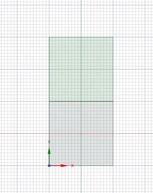
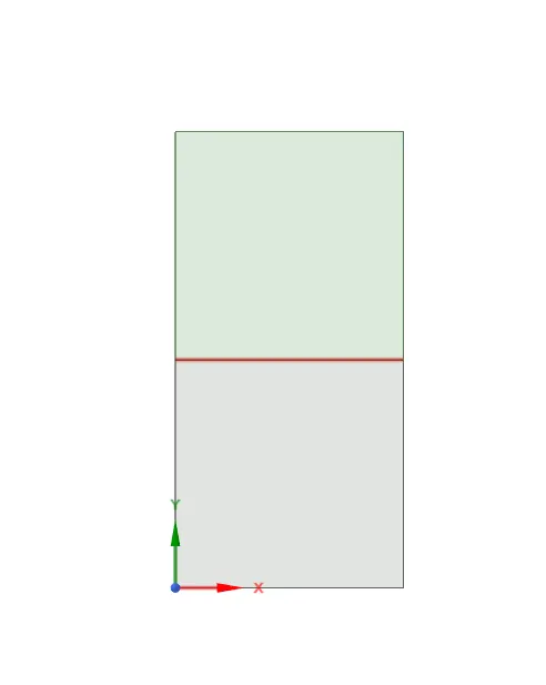
We then use the pull tool to create a surface geometry of the same. Also, we use the share tool to share the topology between the two surfaces and obtain a conformal mesh. We thereby share 1 co-incident edge.
2. MESHING
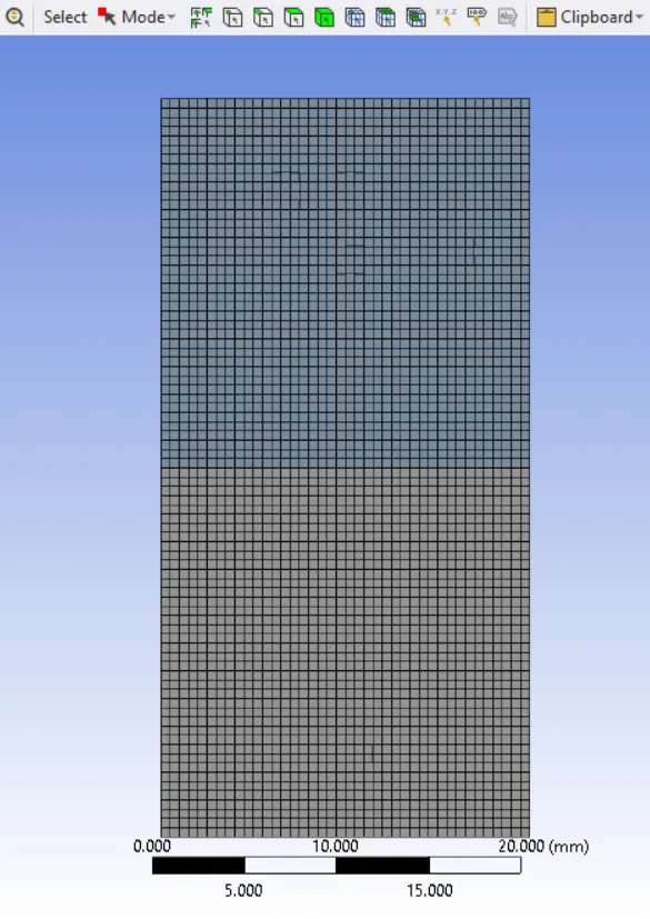
In this step, we are going to generate a base mesh of element size 0.5 mm for the above obtained geometry and observe its characteristics. We obtain the meshing as shown.
3. SETUP & SOLUTION
In this step, we setup the necessary parameters required to run the simulation.
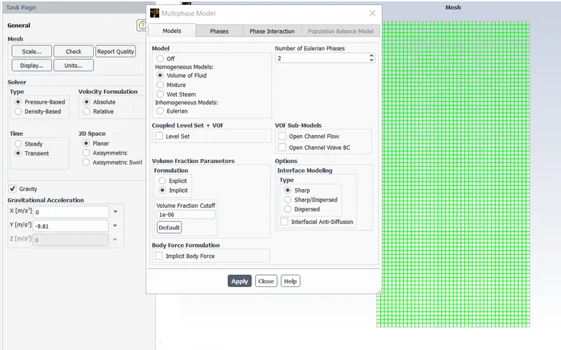
- We use a pressure – based solver with absolute velocity formulation.
- We use a transient state time condition to run the simulation.
- We enable gravity on the negative y – axis with a standard g value of 9.81 `m`/`s^2`.
- We use the laminar viscous model.
- We use a multiphase homogeneous model representing the volume of fluids (VOF)
- 2 Eulerian phases with implicit volume fraction formulation.
- Fluent fluid materials – Air and Water (H2O)
- We consider the first phase (primary) as air and the second phase as water.
- We standard initialize the simulation and create contours of volume fraction and solution animations for the same.
- We patch the two surfaces together with the volume fraction value being ‘1’ for water and ‘0’ for air.
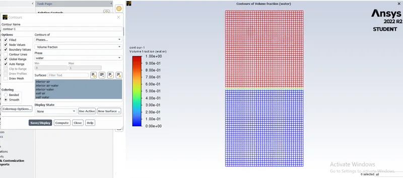
We run the simulation for 600 timesteps, for a timestep size of 0.005 to obtain the following results.
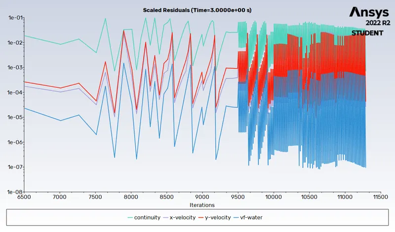
Residuals Plot :
Animation Playback :
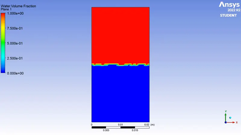
Video Link : https://youtu.be/z-UtyV-xWEE
CASE – 2 : REFINED MESH (element size = 0.2 mm)
In this case setup, we run the simulation for the same parameters by refining the mesh size so as to observe the effects the meshing size has on the simulation.
For the same geometry, we obtain the refined meshing as shown below.
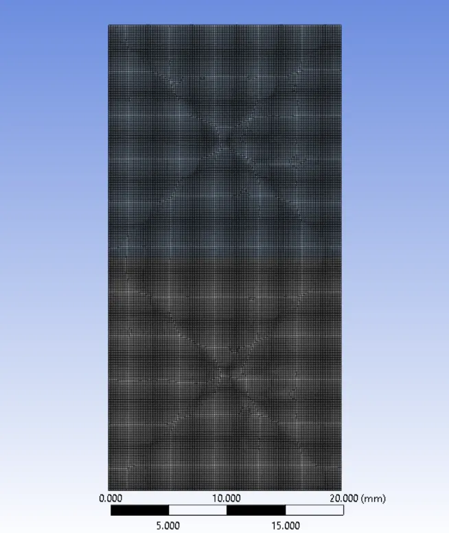
For this meshed geometry, we run the simulation with the same setup parameters for 700 timesteps to obtain the following outputs.
Residuals Plot :
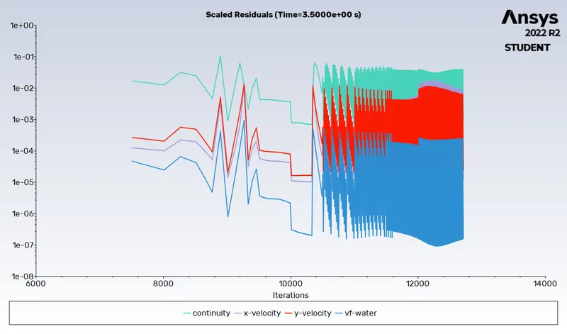
Animation Playback of Simulation :
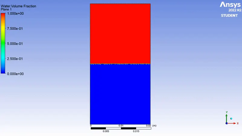
Video Link : https://youtu.be/SH8bwQgkU-w
CASE – 3 : USER – DEFINED MATERIAL (REFINED MESH)
In this case setup, we are going to run the simulation for water and a user-defined material, for a refined mesh.
Specifications of the user – defined material :
Density `rho` = 400 `kg`/`m^3`
Viscosity `mu` = 0.001 `kg`/`m-s`
For this case study, we are going to setup a user-defined material along with water, for the same meshed geometry (element size 0.2 mm). The user-defined material setup is as follows.
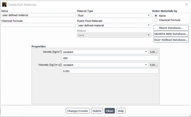
As shown above, we create an user-defined material of density `400` `kg`/`m^3` and viscosity `0.001` `kg`/`m-s`. Furthermore, we create the 2 Eulerian phases as water and user-defined material. We run the calculation for 700 timesteps for a timestep size of 0.005 to obtain the following results.
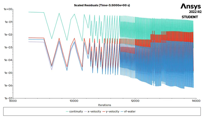
Residuals Plot :
Solution Animation Playback :
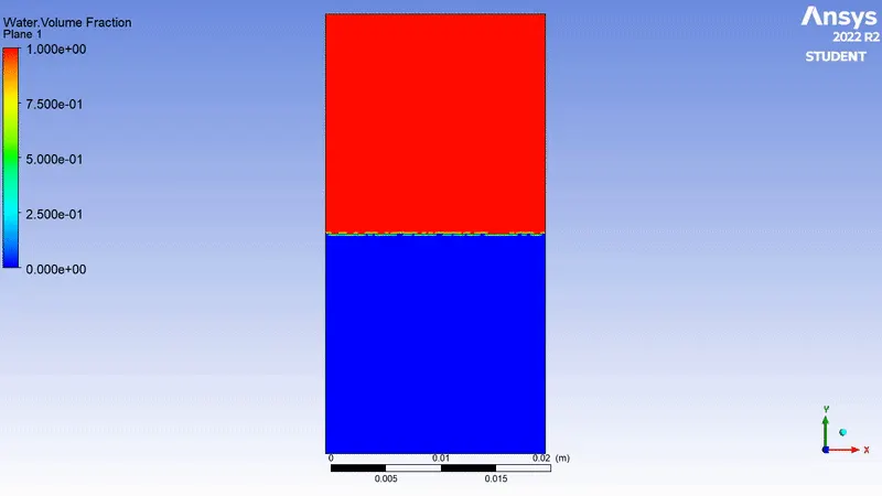
Video Link : https://youtu.be/Lt5LCe_gcvE
ATWOOD NUMBER :
The Atwood number (A) is a dimensionless number in fluid dynamics used in the study of hydrodynamic instabilities in density stratified flows. It is a dimensionless density ratio related to the density of heavier fluid and the density of lighter fluid.
It is a dimensionless density ratio defined as,
`A = (rho_1 – rho_2)/(rho_1 + rho_2)`
Where,
`rho_1` = Density of heavier fluid
`rho_2` = Density of lighter fluid.
Calculating the Atwood number for both the cases,
Cases – 1 & 2 :
Density of heavier fluid (water) `rho_1` = `997` `kg`/`m^3`
Density of lighter fluid (air) `rho_2` = `1.225` `kg`/`m^3`
According to the definition, Atwood number is given by,
`A = (997 – 1.225)/(997 + 1.225)`
Therefore, A = 0.99754
Case – 3 :
Density of heavier fluid (water) `rho_1` = `997` `kg`/`m^3`
Density of lighter fluid (user-defined material) `rho_2` = `400` `kg`/`m^3`
According to the definition, Atwood number is given by,
`A = (997 – 400)/(997 + 400)`
Therefore, A = 0.4273
Atwood number is an important parameter in the study of Rayleigh–Taylor instability. For Atwood number close to 0, RT instability flows take the form of symmetric “fingers” of fluid; for Atwood number close to 1, the much lighter fluid “below” the heavier fluid takes the form of larger bubble-like plumes.
Atwood number has a direct effect on the growth of the petrubations. A higher Atwood number leads to a rapid or non-linear accelerating growth of the interface whereas for a lower Atwood number (closer to 0), leads to a steady growth with bubble like petrubation formation of the interface.
Why is a steady – state approach not suitable for this simulation?
Steady state models are based on the assumptions that all flow conditions and properties of the system are constant with respect to time. Transient models, however, can handle conditions that change with time and assess the time-dependent impact on thermal and flow predictions. Furthermore, transient multiphase flow simulations may become relevant as the conditions change over time.
In this case, a steady state solver can be used for the simulation if only the end result is required. But in this case, we need to study the characteristics of the fluid over a period of time and hence, a time marching solution would be more suitable for this simulation.
CONCLUSIONS & TECHNICAL DISCUSSIONS :
The transient – state simulation for all the three cases, representing the coarse mesh, refined mesh and for a user – defined material has been successfully simulated and the results have been obtained.
From the results, we can observe that a finer meshing results in a much clearer and more defined fluid interface, as it captures the details of the instability much better, as compared to a coarse mesh. It can also be noted that the computational time required for a refined mesh is higher.
For this simulation, a transient – state solver is preferred over a steady – state solver, as it involves variables and instabilities that are captured over a period of time. This gives us an accurate representation of the instabilities forming at the fluid interface in real – time. As a result of this simulation, the time required for the denser fluid to settle down is longer, as compared to that of the lighter fluid.
For the first two cases, we can observe that as the instability forms, finger like petrubations are formed, due to the value of the Atwood number being closer to 1 (0.99754 for cases 1 & 2). Whereas for the third case, we can observe that bubble like plumes are formed at the fluid interface due to the lower Atwood number value (0.4273). Therefore, we can conclude that as the Atwood number value increases (closer to 1), the interface growth is more rapid with finger shaped formations. Whereas, for a smaller Atwood number (closer to 0), we obtain a steady growth with bubble like formations.
Therefore, as the density ratio increases, the interface instability due to the mixing is more rapid.