Week 5.1 - Mid term project - Solving the steady and unsteady 2D heat conduction problem

OBJECTIVES :

1. To solve the 2D heat conduction equation by using the point iterative techniques - Jacobi, Gauss – Seidel and Successive Over Relaxation (SOR) methods.
   
   
2. To implement the above iterative techniques for both Steady State and Transient State Analysis of the equation.
   
   
3. To write a code for both implicit and explicit schemes.

INTRODUCTION :

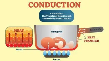
Heat conduction (or thermal conduction) is the transmission of heat from one object to another one that has a different temperature, when they are in direct contact with each other.

Following are the examples of conduction:

• Ironing of clothes is an example of conduction where the heat is conducted from the iron to the clothes.
• Heat is transferred from hands to ice cube resulting in the melting of an ice cube when held in hands.
• Heat conduction through the sand at the beaches. This can be experienced during summers. Sand is a good conductor of heat.

2 – D Heat Conduction Equation :

Considering the general 3-D Heat Conduction Equation containing both the Time Derivative and Spatial Derivative terms,

`(delT)/(delt) + alpha((del^2T)/(delx^2) + (del^2T)/(dely^2) + (del^2T)/(delz^2)) = 0`

Now, considering the above equation for a 2-D plane or space. As it is 2 dimensional, the Z-axis does not come into consideration.

Thereby, the general 2-D form of the Heat Conduction Equation is given by,

`(delT)/(delt) + alpha((del^2T)/(delx^2) + (del^2T)/(dely^2)) = 0`

Where, `alpha` = Thermal Diffusivity (`m^2`/s)

We are going to solve the above equation using two approaches.

1. Transient Equation Form :
   During any period in which temperatures changes in time at any place within an object, the mode of thermal energy flow is termed transient conduction. Another term is "non-steady-state" conduction, referring to the time-dependence of temperature fields in an object.

The Transient form of the 2-D Heat Conduction Equation is given by,

`(delT)/(delt) + alpha((del^2T)/(delx^2) + (del^2T)/(dely^2)) = 0` or `(delT)/(delt) + alpha(nablaT) = 0`

Where, `nablaT` = Laplacian of T.

2. Steady State Equation Form :
   Steady-state conduction is the form of conduction that happens when the temperature difference driving the conduction is constant, so that after an equilibration time, the spatial distribution of temperatures in the conducting object does not change any further. In steady-state conduction, the amount of heat entering any region of an object is equal to the amount of heat coming out (if this were not so, the temperature would be rising or falling, as thermal energy was tapped or trapped in a region).

The Steady State form of the 2-D Heat Conduction Equation is given by,

`(del^2T)/(delx^2) + (del^2T)/(dely^2) = 0` or `nabla^2T = 0`

We are going to be solving the above forms of equations with the help of 3 iterative techniques. They are,

1. Jacobi Method :
   Jacobi method is an iterative algorithm for determining the solutions of a strictly diagonally dominant system of linear equations. Each diagonal element is solved and an approximate value is plugged in. The process is then iterated until it converges.

The element-based formula for Jacobi method is,

Where, `x^k` is the `k^(th)` approximation or iteration of `x` and `x^(k+1)` is the next or `k + 1^(th)` iteration of `x`.

2. Gauss – Seidel Method :
   Gauss–Seidel method, also known as the Liebmann method or the method of successive displacement, is an iterative method used to solve a system of linear equations and is similar to the Jacobi method. Though it can be applied to any matrix with non-zero elements on the diagonals, convergence is only guaranteed if the matrix is either strictly diagonally dominant or symmetric and positive definite.
   
   The element-based formula for Gauss – Seidel method is,

3. Successive Over Relaxation (SOR) Method :
   The method of successive over-relaxation (SOR) is a variant of the Gauss–Seidel method for solving a linear system of equations, resulting in faster convergence. It is kind of a wrapper or more of an enhancer, which can enhance the performance of Jacobi or Gauss – Seidel methods.

The formula for SOR method is,

Where, `omega` = Relaxation Factor and depends upon the properties of the coefficient matrix.

GIVEN DATA AND ASSUMPTIONS :

1. Assume that the domain is a unit square of length 1m.
   
   
2. Assume uniform number of grid points along the x – axis as well as on the y – axis (nx = ny).
   
   
3. The boundary conditions for the Steady and Transient State are given as,
   i.) Left = 400K
   ii.) Top = 600K
   iii.) Right = 800K
   iv.) Bottom = 900K
   
   
4. The absolute error criteria is `1e^-4`.
   
   
5. Starting error = `9e^9`.
   
   
6. Relaxation factor for SOR method `omega` = 1.2.
   
   
7. Thermal Diffusivity, `alpha = 1.88e^-5`.
   
   
8. CFL Number Criteria, `"CFL Number" <= 0.5`

STEADY STATE EQUATION :

We have the Steady State form of the 2-D Heat Conduction Equation as,

`(del^2T)/(delx^2) + (del^2T)/(dely^2) = 0` or `nabla^2T = 0`

Discretizing the above equation using the Central Differencing Scheme, we get

`(T_L - 2T_P + T_R)/(Deltax^2) + (T_T - 2T_P + T_B)/(Deltay^2) = 0`

On simplifying the above equation, we get

`T_P = 1/k((T_L + T_R)/(Deltax^2) + (T_T + T_B)/(Deltay^2))` We have assumed `k = (2(Deltax^2 + Deltay^2))/(Deltax^2.Deltay^2)`

Where,

`T_P` = Current Point

`T_R` = Right Point

`T_L` = Left Point

`T_T` = Top Point

`T_B` = Bottom Point.

Function Code for Jacobi Method (Steady State):

function T = jacobi_iteration(nx,ny,error,tolerance,xx,yy,dx,dy,T,k,T_old);

jacobi_iteration = 1;

% Convergence loop
while error>tolerance
    for i = 2:nx-1
        for j = 2:ny-1

            term_1 = (T_old(i-1,j) + T_old(i+1,j))/(k*(dx^2));
            term_2 = (T_old(i,j-1) + T_old(i,j+1))/(k*(dy^2));
            T(i,j) = term_1 + term_2;

        end
    end

    error = max(max(abs(T_old - T)));
    T_old = T;
    jacobi_iteration = jacobi_iteration + 1;

    % Plotting
    figure(1)
    [A,B] = contourf(xx,yy,T);
    colormap("jet")
    set(gca,'YDir','reverse')
    colorbar
    title_text = sprintf('Jacobi Iteration Number = %d',jacobi_iteration);
    title(title_text)
    xlabel('x')
    ylabel('U')
    clabel(A,B)
    pause(0.03)
end
fprintf('Number of Iterations for Jacobi = %d',jacobi_iteration)
end

Function Code for Gauss - Seidel Method (Steady State):

function T = gauss_seidel_iteration(nx,ny,error,tolerance,xx,yy,dx,dy,T,k,T_old);

gauss_seidel_iteration = 1;

% Convergence loop
while error>tolerance
    for i = 2:nx-1
        for j = 2:ny-1

            term_1 = (T(i-1,j) + T_old(i+1,j))/(k*(dx^2));
            term_2 = (T(i,j-1) + T_old(i,j+1))/(k*(dy^2));
            T(i,j) = term_1 + term_2;

        end
    end

    error = max(max(abs(T_old - T)));
    T_old = T;
    gauss_seidel_iteration = gauss_seidel_iteration + 1;

    % Plotting
    figure(2)
    [C,D] = contourf(xx,yy,T);
    colormap("jet")
    set(gca,'YDir','reverse')
    colorbar
    title_text = sprintf('Gauss - Seidel Iteration Number = %d',gauss_seidel_iteration);
    title(title_text)
    xlabel('x')
    ylabel('U')
    clabel(C,D)
    pause(0.03)
end
fprintf('Number of Iterations for Gauss - Seidel = %d',gauss_seidel_iteration)
end

Function Code for SOR Method (Steady State):

function T = SOR_iteration(nx,ny,error,tolerance,xx,yy,dx,dy,T,k,T_old);

SOR_iteration = 1;
omega = 1.2;

% Convergence loop
while error>tolerance
    for i = 2:nx-1
        for j = 2:ny-1

            term_1 = (T(i-1,j) + T_old(i+1,j))/(k*(dx^2));
            term_2 = (T(i,j-1) + T_old(i,j+1))/(k*(dy^2));
            T_gs = term_1 + term_2;
            T(i,j) = ((1-omega)*T_old(i,j)) + (omega*T_gs);

        end
    end

    error = max(max(abs(T_old - T)));
    T_old = T;
    SOR_iteration = SOR_iteration + 1;

    % Plotting
    figure(3)
    [E,F] = contourf(xx,yy,T);
    colormap("jet")
    set(gca,'YDir','reverse')
    colorbar
    title_text = sprintf('SOR Iteration Number = %d',SOR_iteration);
    title(title_text)
    xlabel('x')
    ylabel('U')
    clabel(E,F)
    pause(0.03)
end
fprintf('Number of Iterations for SOR = %d',SOR_iteration)
end

Function Code Explanation :

1. We first begin the function code by defining the function handle, representing the respective Jacobi, Gauss – Seidel and SOR iteration methods and assigning them to an output array “T”.
   
   This function takes the respective inputs being,
   i.) Number of grid points along x-axis (nx).
   ii.) Number of grid points along y-axis (ny).
   iii.) Error.
   iv.) Absolute error criteria (tolerance).
   v.) “xx” and “yy” arrays obtained by using the meshgrid function for x and y values.
   vi.) Grid spacing on the x-axis (dx), which is the difference between the consecutive values of x.
   vii.) Grid spacing on the y-axis (dy), which is the difference between the consecutive values of y.
   viii.) The arrays “T” and “T_old”.
   ix.) The calculated value “k”.
   
   
   
   
2. In the next step, we define the initial iteration number, which we are going to increase by a value of 1 after running each loop. The iterations keep running over and over again till the error drops below the respective tolerance limit.
   
   For the SOR method, we define the value of the relaxation factor (omega), which will be used further on.
   
   
   
   
   
3. Next, we create a convergence loop, with the while condition that it keeps looping till the error value drops below the tolerance limit. In this loop, we create two for loops for the range of nodes excluding the boundary nodes (as their value is already known). These two for loops include the discretized equation in the form of nodes.
   
   These equations are as follows,
   For Jacobi Method,
   
   `T(i,j) = 1/k[(T_(old)(i-1,j) + T_(old)(i+1,j))/(Deltax^2) + (T_(old)(i,j-1) + T_(old)(i,j+1))/(Deltay^2]]`
   
   
   
   For Gauss – Seidel Method,
   
   `T(i,j) = 1/k[(T(i-1,j) + T_(old)(i+1,j))/(Deltax^2) + (T(i,j-1) + T_(old)(i,j+1))/(Deltay^2]]`
   
   
   
   For SOR Method,
   
   `T(i,j) = (1-omega)T_(old)(i,j) + omega[1/k((T(i-1,j) + T_(old)(i+1,j))/(Deltax^2) + (T(i,j-1) + T_(old)(i,j+1))/(Deltay^2])]`
   
   
   
   
   
4. After the loops have been run for the respective number of times, we then calculate the error values obtained, by calculating the maximum absolute difference between the T_old matrix and the new updated T matrix.
   
   Also, we update the new calculated values to the T_old matrix and move on to the next iteration by raising the iteration value by a factor of 1 after each loop.
   
   
   
   
   
5. Finally, a contour plot is obtained from the values of xx , yy and T matrix to which we provide the respective colour codes and colour bars. We use the “set” command to reverse the direction of the y – axis as required.
   
   This contour plot represents the 2-D Heat Conduction Equation for the various iterative methods ( Jacobi , Gauss – Seidel and SOR Methods ) and how the number of iterations vary with respect to each method.
   

Final Program Code (Steady State):

% STEADY STATE EQUATION FORM
clear all
close all
clc


% INPUTS
% Domain is an unit square of length 1m
L = 1;

% Number of grid points along x-axis
nx = 10;

% Number of grid points along y-axis
ny = nx;

% Absolute error criteria
tolerance = 1e-5;

% Error (should be greater than tolerance)
error = 9e9;



% X and Y axis mesh
x = linspace(0,L,nx);
y = linspace(0,L,ny);
[xx,yy] = meshgrid(x,y);

% Grid spacing
dx = x(2)-x(1);
dy = y(2)-y(1);

% Initializing Temperature matrix
T = ones(nx,ny);

% Defining boundary conditions
T_L = 400;
T_T = 600;
T_R = 800;
T_B = 900;

% Creating the unit square matrix from BC
% Initializing temperature

T(:,1) = T_L;
T(1,:) = T_T;
T(:,end) = T_R;
T(end,:) = T_B;

% Average temperature at the corner of the matrix
T(1,1) = (T_T + T_L)/2;
T(1,end) = (T_T + T_R)/2;
T(end,end) = (T_R + T_B)/2;
T(end,1) = (T_B + T_L)/2;

% Additionals
T_old = T;
k = 2*((dx^2) + (dy^2))/((dx^2)*(dy^2));



% DEFINING THE SOLVERS
iterative_solver = input('Enter number wrt solver :')

if iterative_solver == 1;
    tic;
    T_jacobi = jacobi_iteration(nx,ny,error,tolerance,xx,yy,dx,dy,T,k,T_old);
    jacobi_time = toc;

elseif iterative_solver == 2;
    tic;
    T_gauss_seidel = gauss_seidel_iteration(nx,ny,error,tolerance,xx,yy,dx,dy,T,k,T_old);
    gauss_seidel_time = toc;

elseif iterative_solver == 3;
    tic;
    T_SOR = SOR_iteration(nx,ny,error,tolerance,xx,yy,dx,dy,T,k,T_old);
    SOR_time = toc;
end

Final Program Code Explanation :

1. We begin the program by using the clear all, close all and clc commands to clear up the command window as well as the workspace.
   
   
   
   
2. In the next step, we define all the input values, which are being considered in the program.
   
   The inputs are as follows,
   i.) Length of domain unit square, L = 1m.
   ii.) Number of grid points along x and y – axes, nx = ny = 10.
   iii.) Absolute error criteria, tolerance = 1e-5.
   iv.) Assumed error (which should be greater than tolerance), error = 9e9.
   
   
   
   
3. Next, we create the x and y arrays, representing the number of nodes on the x and y – axes, by using the linspace command to obtain “nx or ny” number of equally distributed values between 0 and L.
   
   From these values of x and y, we create a mesh by using the meshgrid command to obtain the final matrix of xx and yy, which is the unit square matrix. Also, we calculate the grid spacing values (dx and dy) by calculating the difference between the corresponding values of x or y.
   
   
   
   
4. In the next step, we assume the initial guess matrix of T as an array of all ones (using the ones command) for nx and ny number of rows and columns. To this guess matrix, we define the provided Boundary Conditions to the respective top , right , left and bottom boundaries of the unit square.
   
   Also, we calculate the corner values of the matrix by taking the average of the two boundaries it is in contact with and therefore, we obtain the final guess matrix with the boundary conditions defined.
   
   
   
   
5. Additionally, we update these new values to the matrix T and also calculate the value of “k” which we have assumed from the derivation as,
   
   `k = (2(Deltax^2 + Deltay^2))/(Deltax^2.Deltay^2)`
   
   
   
   
   
6. Finally, we include all the function codes of the Jacobi , Gauss – Seidel and SOR methods respectively in an “if” and “elseif” function such that if we input the iterative solver number as 1 in the command prompt, the function code for Jacobi method is run and similarly, 2 for Gauss – Seidel and 3 for SOR method.
   
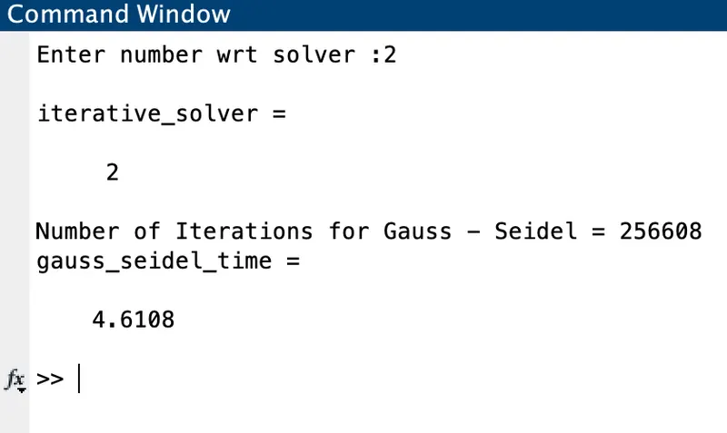
   Thereby, we obtain the respective contour plots for all the 3 iterative methods and the number of iterations carried out for each method as well as the simulation time is noted down and compared.

Steady State Outputs :

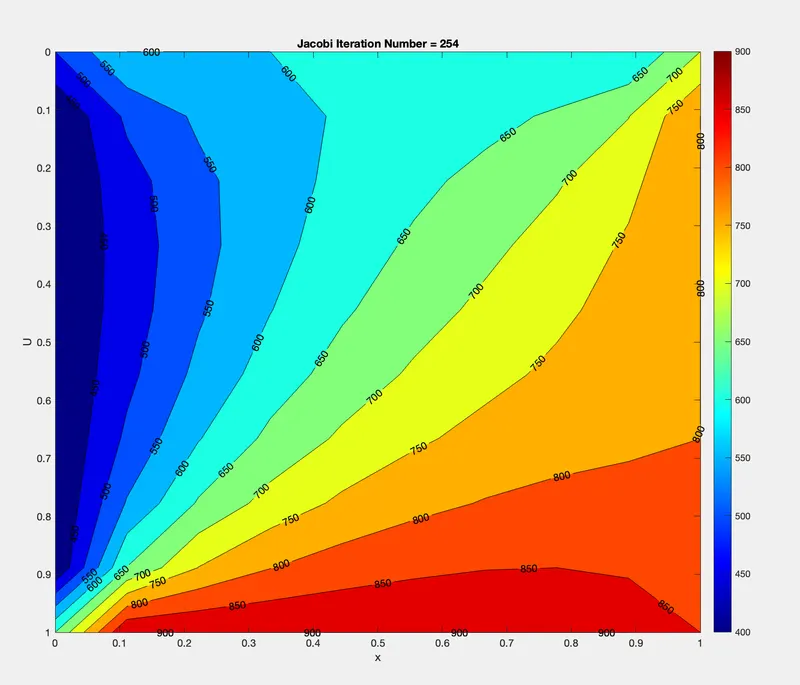
1. Jacobi Method :
   
   
   Contour Plot :
   
   
   
   
   
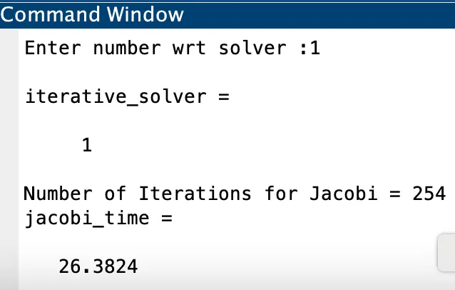
   Number of Iterations and Simulation Time :
   
   
   
   
   
   
   
   
   
   
   
   
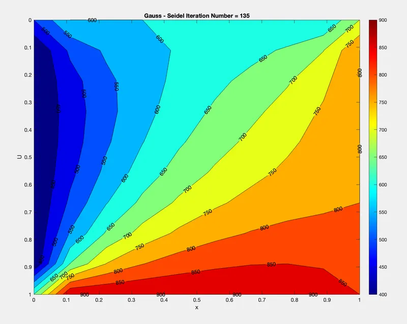
2. Gauss - Seidel Method :
   
   
   Contour Plot :
   
   
   
   
   
   
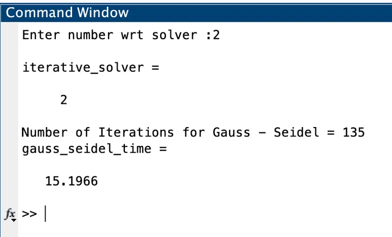
   Number of Iterations and Simulation Time :
   
   
   
   
   
   
   
   
   
   
   
   
3. Successive - Over Relaxation (SOR) Method :
   
   
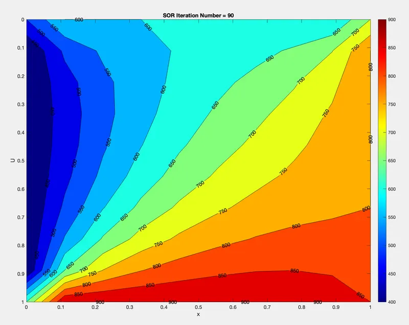
   Contour Plot :
   
   
   
   
   
   
   
   Number of Iterations and Simulation Time :
   
   

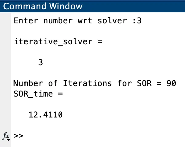
From the above plots, we can observe that the SOR iterative method requires the least number of iterations and the least simulation time as well. Thereby, this method is the fastest when compared to the other two iterative methods.

TRANSIENT STATE EQUATION (UNSTEADY STATE):

The Transient form of the 2-D Heat Conduction Equation is given by,

`(delT)/(delt) + alpha((del^2T)/(delx^2) + (del^2T)/(dely^2)) = 0` or `(delT)/(delt) + alpha(nablaT) = 0`

Where,

`nablaT` = Laplacian of T.

`alpha` = Thermal Diffusivity (`m^2`/s)

We are going to solve the above equation in 2 approaches, being the Explicit Method and Implicit Method.

Explicit Method for Transient State (Unsteady State):

Explicit method is an approach used in numerical analysis for obtaining numerical approximations to the solutions of time-dependent ordinary and partial differential equations, as is required in computer simulations of physical processes. Explicit methods calculate the state of a system at a later time from the state of the system at the current time.

In this method, each differential equation contains one unknown function, which can be solved for using this method.

Discretizing the above Transient Equation Form by employing Central Difference Scheme for the second order derivative terms,

Therefore, the discretized terms are as follows.

`(delT)/(delt) = (T^(n+1)(i,j) - T^n(i,j))/(Deltat)`

`(del^2T)/(delx^2) = (T^n(i+1,j) - 2T^n(i,j) + T^n(i-1,j))/(Deltax^2)`

`(del^2T)/(dely^2) = (T^n(i,j+1) - 2T^n(i,j) + T^n(i,j-1))/(Deltay^2)`

We obtain a pair of uncoupled linear equations which we are further going to solve. Substituting these discretized equation in the Transient Equation and simplifying, we get,

`T^(n+1)(i,j) = T^n(i,j) + alpha.Deltat[(T^n(i+1,j) - 2T^n(i,j) + T^n(i-1,j))/(Deltax^2) + (T^n(i,j+1) - 2T^n(i,j) + T^n(i,j-1))/(Deltay^2)]`

Introducing variables `k_1` and `k_2` to simplify the above equation. These variables are known as CFL Numbers.

`k_1 = (alpha.Deltat)/(Deltax^2)` and `k_2 = (alpha.Deltat)/(Deltay^2)`

`therefore` `T^(n+1)(i,j) = T^n(i,j) + k_1[T_(old)^n(i+1,j) - 2T_(old)^n(i,j) + T_(old)^n(i-1,j)] + k_2[T_(old)^n(i,j+1) - 2T_(old)^n(i,j) + T_(old)^n(i,j-1)]`

Function Code for Transient State using Explicit Method :

function T = transient_explicit(nx,ny,nt,xx,yy,T,k1,k2,T_old);

looping_term = 1;

% Convergence loop
for k = 1:nt;
    for i = 2:nx-1
        for j = 2:ny-1

            term_1 = T_old(i,j);
            term_2 = k1*(T_old(i+1,j) - (2*T_old(i,j)) + T_old(i-1,j));
            term_3 = k2*(T_old(i,j+1) - (2*T_old(i,j)) + T_old(i,j-1));
            T(i,j) = term_1 + term_2 + term_3;

        end
    end

    error = max(max(abs(T_old - T)));
    T_old = T;
    looping_term = looping_term + 1;
end


    % Plotting
    figure(1)
    [A,B] = contourf(xx,yy,T);
    colormap("jet")
    set(gca,'YDir','reverse')
    colorbar
    title_text = sprintf('Number of Counters = %d',looping_term);
    title(title_text)
    xlabel('x')
    ylabel('U')
    clabel(A,B)
    pause(0.03)

fprintf('Number of Counters = %d',looping_term)
end

Final Program Code for Transient State using Explicit Method :

% TRANSIENT STATE EQUATION FORM (EXPLICIT METHOD)
clear all
close all
clc


% INPUTS
% Domain is an unit square of length 1m
L = 1;

% Number of grid points along x-axis
nx = 40;

% Number of grid points along y-axis
ny = nx;

% Absolute error criteria
tolerance = 1e-5;

% Error (should be greater than tolerance)
error = 9e9;

% Time Limit (in seconds)
time_limit = 1200;

% Time Step (in seconds)
dt = 0.01;

% Number of Time Steps
nt = time_limit/dt;

% Thermal Diffusivity (in m^2/s)
alpha = 1.88e-5;



% X and Y axis mesh
x = linspace(0,L,nx);
y = linspace(0,L,ny);
[xx,yy] = meshgrid(x,y);

% Grid spacing
dx = x(2)-x(1);
dy = y(2)-y(1);

% Initializing guess matrix
T = ones(nx,ny);

% Defining boundary conditions
T_L = 400;
T_T = 600;
T_R = 800;
T_B = 900;

% Creating the unit square matrix from BC
% Initializing temperature

T(:,1) = T_L;
T(1,:) = T_T;
T(:,end) = T_R;
T(end,:) = T_B;

% Average temperature at the corner of the matrix
T(1,1) = (T_T + T_L)/2;
T(1,end) = (T_T + T_R)/2;
T(end,end) = (T_R + T_B)/2;
T(end,1) = (T_B + T_L)/2;

% Additionals
T_old = T;
k1 = alpha*(dt/(dx^2));
k2 = alpha*(dt/(dy^2));



% DEFINING THE SOLVERS
solver = input('Enter number wrt solver :')

if solver == 1;
    tic
    T_explicit = transient_explicit(nx,ny,nt,xx,yy,T,k1,k2,T_old);
    time = toc
end

Outputs for Transient State using Explicit Method :

Contour Plot :

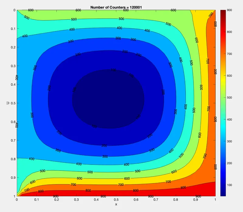
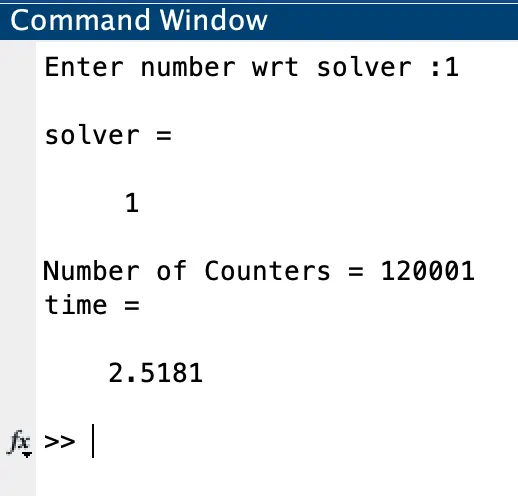
Number of Iterations and Simulation Time :

Implicit Method for Transient State (Unsteady State):

Implicit methods are approaches used in numerical analysis for obtaining numerical approximations to the solutions of time-dependent ordinary and partial differential equations, as is required in computer simulations of physical processes. Implicit methods find a solution by solving an equation involving both the current state of the system (n) and the later one (n+1).

Discretizing the Transient Equation Form by employing Central Difference Scheme for the second order derivative terms,

Therefore, the discretized terms are as follows.

`(delT)/(delt) = (T^(n+1)(i,j) - T^n(i,j))/(Deltat)`

`(del^2T)/(delx^2) = (T^(n+1)(i+1,j) - 2T^(n+1)(i,j) + T^(n+1)(i-1,j))/(Deltax^2)`

`(del^2T)/(dely^2) = (T^(n+1)(i,j+1) - 2T^(n+1)(i,j) + T^(n+1)(i,j-1))/(Deltay^2)`

We obtain a pair of uncoupled linear equations which we are further going to solve. Substituting these discretized equation in the Transient Equation and simplifying, we get,

`T^(n+1)(i,j) = T^n(i,j) + alpha.Deltat[(T^(n+1)(i+1,j) - 2T^(n+1)(i,j) + T^(n+1)(i-1,j))/(Deltax^2) + (T^(n+1)(i,j+1) - 2T^(n+1)(i,j) + T^(n+1)(i,j-1))/(Deltay^2)]`

Introducing variables `k_1` and `k_2` to simplify the above equation,

`k_1 = (alpha.Deltat)/(Deltax^2)` and `k_2 = (alpha.Deltat)/(Deltay^2)`

`T^(n+1)(i,j) = T^n(i,j) + k_1[T_(old)^(n+1)(i+1,j) - 2T_(old)^(n+1)(i,j) + T_(old)^(n+1)(i-1,j)] + k_2[T_(old)^(n+1)(i,j+1) - 2T_(old)^(n+1)(i,j) + T_(old)^(n+1)(i,j-1)]`

Simplifying the above equation, we get,

`T^(n+1)(i,j) = 1/(1+2k_1+2k_2).[T^n(i,j) + k_1[T_(old)^(n+1)(i+1,j) + T_(old)^(n+1)(i-1,j)] + k_2[T_(old)^(n+1)(i,j+1) + T_(old)^(n+1)(i,j-1)]]`

Thereby, spllitting the above equation into 3 terms.

Term 1 = `1/(1+2k_1+2k_2)`

Term 2 = `k_1`. Term 1

Term 3 = `k_2` . Term 1

Therefore, the final equation becomes,

`T^(n+1)(i,j) = "Term 1"* T^n(i,j) + "Term 2"*[T^(n+1)(i+1,j) + T^(n+1)(i-1,j)] + "Term 3"*[T^(n+1)(i,j+1) + T^(n+1)(i,j-1)]`

We are going to solve the above equation using 3 iterative methods,

1. Jacobi Iteration Method :

For the Jacobi Iteration Method, we first assume a guess matrix for the unknown (n+1) terms. With the help of these assumed values, the equation is solved to obtain the new updated values of the guess matrix and it is further compared with the previous values. This step is carried out for a respective number of times, till the error between the two compared matrices drop below the threshold limit or tolerance. This obtained value which is below the error tolerance limit is used to obtain the solutions at the next time steps and so on and thereby, the final solution is obtained.

Function Code for Jacobi Method for Transient State (Implicit Method) :

function T = jacobi_transient_implicit(nx,ny,nt,tolerance,xx,yy,T,k1,k2,T_old,T_prev_dt);

jacobi_iteration = 1;

% Time loop
for k = 1:nt;
    error = 9e9;

    % Convergence Loop
    while error>tolerance
    for i = 2:nx-1
        for j = 2:ny-1

            term_1 = (1 + (2*k1) + (2*k2))^-1;
            term_2 = k1 * term_1;
            term_3 = k2 * term_1;
            H = (T_old(i-1,j) + T_old(i+1,j));
            V = (T_old(i,j-1) + T_old(i,j+1));
            T(i,j) = (T_prev_dt(i,j)*term_1) + (term_2*H) + (term_3*V);

        end
    end

    error = max(max(abs(T_old - T)));
    T_old = T;
    jacobi_iteration = jacobi_iteration + 1;
    end
    T_prev_dt = T;
end


    % Plotting
    figure(1)
    [A,B] = contourf(xx,yy,T);
    colormap("jet")
    set(gca,'YDir','reverse')
    colorbar
    title_text = sprintf('Jacobi Iteration Number = %d',jacobi_iteration);
    title(title_text)
    xlabel('x')
    ylabel('U')
    clabel(A,B)
    pause(0.03)

fprintf('Number of Iterations for Jacobi = %d',jacobi_iteration)
end

2. Gauss - Seidel Method :

Gauss - Seidel iteration is similar to that of the Jacobi method but instead of using the old values (`T_(old)`) of the guess matrix to calculate the values for the next time step, we use the new updated values (`T`) for the same.

Function Code for Gauss - Seidel Method for Transient State (Implicit Method) :

function T = gauss_seidel_transient_implicit(nx,ny,nt,tolerance,xx,yy,T,k1,k2,T_old,T_prev_dt);

gauss_seidel_iteration = 1;

% Time loop
for k = 1:nt;
    error = 9e9;

    % Convergence Loop
    while error>tolerance
    for i = 2:nx-1
        for j = 2:ny-1

            term_1 = (1 + (2*k1) + (2*k2))^-1;
            term_2 = k1 * term_1;
            term_3 = k2 * term_1;
            H = (T(i-1,j) + T_old(i+1,j));
            V = (T(i,j-1) + T_old(i,j+1));
            T(i,j) = (T_prev_dt(i,j)*term_1) + (term_2*H) + (term_3*V);

        end
    end

    error = max(max(abs(T_old - T)));
    T_old = T;
    gauss_seidel_iteration = gauss_seidel_iteration + 1;
    end
    T_prev_dt = T;
end


    % Plotting
    figure(2)
    [A,B] = contourf(xx,yy,T);
    colormap("jet")
    set(gca,'YDir','reverse')
    colorbar
    title_text = sprintf('Gauss - Seidel Iteration Number = %d',gauss_seidel_iteration);
    title(title_text)
    xlabel('x')
    ylabel('U')
    clabel(A,B)
    pause(0.03)

fprintf('Number of Iterations for Gauss - Seidel = %d',gauss_seidel_iteration)
end

3. Successive - Over Relaxation (SOR) Method :

This method can be applied for either Jacobi or Gauss - Seidel Methods and is more of an enhancer. This method results in faster convergence.

Function Code for Successive - Over Relaxation (SOR) Method for Transient State (Implicit Method) :

function T = SOR_transient_implicit(nx,ny,nt,tolerance,xx,yy,T,k1,k2,T_old,T_prev_dt);

SOR_iteration = 1;
omega = 1.2;

% Time loop
for k = 1:nt;
    error = 9e9;

    % Convergence Loop
    while error>tolerance
    for i = 2:nx-1
        for j = 2:ny-1

            term_1 = (1 + (2*k1) + (2*k2))^-1;
            term_2 = k1 * term_1;
            term_3 = k2 * term_1;
            H = (T(i-1,j) + T_old(i+1,j));
            V = (T(i,j-1) + T_old(i,j+1));
            T(i,j) = (omega*((T_prev_dt(i,j)*term_1) + (term_2*H) + (term_3*V))) + ((1-omega)*T_prev_dt(i,j));

        end
    end

    error = max(max(abs(T_old - T)));
    T_old = T;
    SOR_iteration = SOR_iteration + 1;
    end
    T_prev_dt = T;
end


    % Plotting
    figure(3)
    [A,B] = contourf(xx,yy,T);
    colormap("jet")
    set(gca,'YDir','reverse')
    colorbar
    title_text = sprintf('SOR Iteration Number = %d',SOR_iteration);
    title(title_text)
    xlabel('x')
    ylabel('U')
    clabel(A,B)
    pause(0.03)

fprintf('Number of Iterations for SOR = %d',SOR_iteration)
end

Final Program Code for Transient State Equation (Implicit Method) :

% TRANSIENT STATE EQUATION FORM (IMPLICIT METHOD)
clear all
close all
clc


% INPUTS
% Domain is an unit square of length 1m
L = 1;

% Number of grid points along x-axis
nx = 40;

% Number of grid points along y-axis
ny = nx;

% Absolute error criteria
tolerance = 1e-5;

% Error (should be greater than tolerance)
error = 9e9;

% Time Limit (in seconds)
time_limit = 1200;

% Time Step (in seconds)
dt = 0.01;

% Number of Time Steps
nt = time_limit/dt;

% Thermal Diffusivity (in m^2/s)
alpha = 1.88e-5;



% X and Y axis mesh
x = linspace(0,L,nx);
y = linspace(0,L,ny);
[xx,yy] = meshgrid(x,y);

% Grid spacing
dx = x(2)-x(1);
dy = y(2)-y(1);

% Initializing guess matrix
T = ones(nx,ny);

% Defining boundary conditions
T_L = 400;
T_T = 600;
T_R = 800;
T_B = 900;

% Creating the unit square matrix from BC
% Initializing temperature

T(:,1) = T_L;
T(1,:) = T_T;
T(:,end) = T_R;
T(end,:) = T_B;

% Average temperature at the corner of the matrix
T(1,1) = (T_T + T_L)/2;
T(1,end) = (T_T + T_R)/2;
T(end,end) = (T_R + T_B)/2;
T(end,1) = (T_B + T_L)/2;

% Additionals
T_old = T;
T_prev_dt = T_old;
k1 = alpha*(dt/(dx^2));
k2 = alpha*(dt/(dy^2));
omega = 2/(1+sin(pi*dx));
CFL = alpha*(dt/(dx^2));



% DEFINING THE SOLVERS
iterative_solver = input('Enter number wrt solver :')

if iterative_solver == 1;
    tic
    T_jacobi_implicit = jacobi_transient_implicit(nx,ny,nt,tolerance,xx,yy,T,k1,k2,T_old,T_prev_dt);
    jacobi_time = toc

elseif iterative_solver == 2;
    tic
    T_gauss_seidel_implicit = gauss_seidel_transient_implicit(nx,ny,nt,tolerance,xx,yy,T,k1,k2,T_old,T_prev_dt);
    gauss_seidel_time = toc

elseif iterative_solver == 3;
    tic
    T_SOR_implicit = SOR_transient_implicit(nx,ny,nt,tolerance,xx,yy,T,k1,k2,T_old,T_prev_dt);
    SOR_time = toc
end

Transient State Outputs (Implicit Method) :

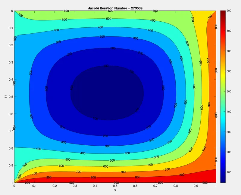
1. Jacobi Iteration Method

Contour Plot :

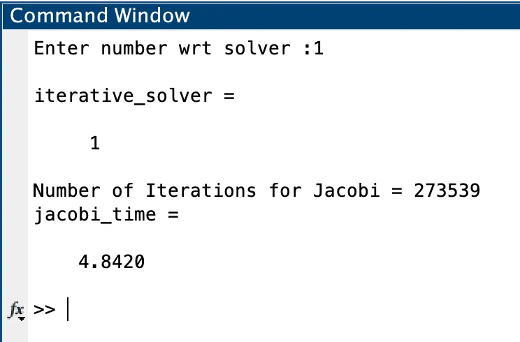
Number of Iterations and Simulation Time :

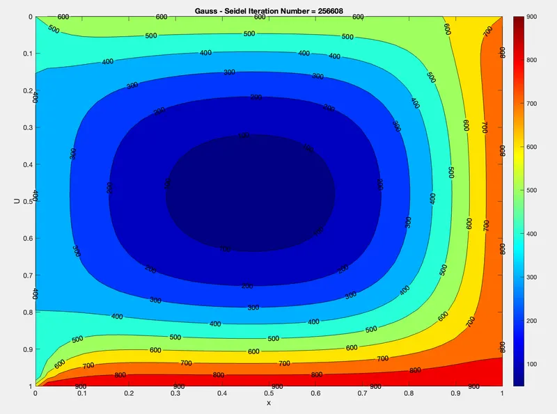
2. Gauss - Seidel Iteration Method

Contour Plot :

Number of Iterations and Simulation Time :

3. Successive - Over Relaxation (SOR) Iteration Method

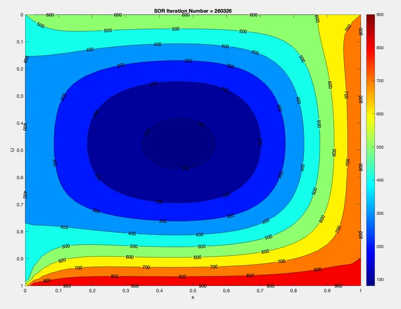
Contour Plot :

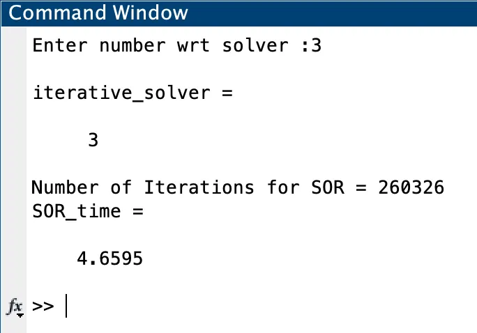
Number of Iterations and Simulation Time :

CONCLUSION :

The respective program codes for the Steady State Equation form and the Transient Equation form of the 2-D Heat Conduction Equation, using the 3 iterative techniques – Jacobi , Gauss – Seidel and Successive Over Relaxation (SOR) methods have been written and thereby, the 2-D Heat Conduction Equation has been solved using both the Explicit and Implicit methods as shown.

From the results, we can observe that the Jacobi iterative method requires the most number of iterations to solve the equation, resulting in a much longer simulation time when compared to the other two iterative methods. Whereas, the SOR iterative method requires the least number of iterations for the same as well as the least simulation time to run, thereby leading to faster convergence.

Thereby, we can conclude that the SOR iteration method is the fastest and most efficient when compared to Jacobi and Gauss – Seidel iteration methods, to solve the 2-D Heat Conduction Equation.

Therefore, SOR < Gauss – Seidel < Jacobi