Project 2 - Rankine cycle Simulator
OBJECTIVES :
- Create a Rankine Cycle Simulator and calculate the state points of cycle based on user inputs.
- Extract steam and water properties from the Xsteam library to calculate the points inbetween state variables.
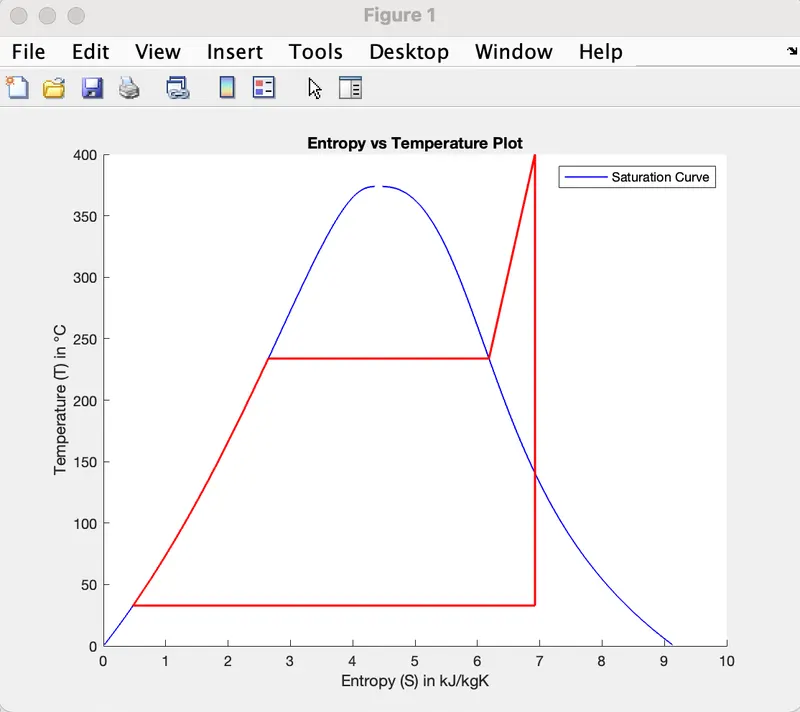
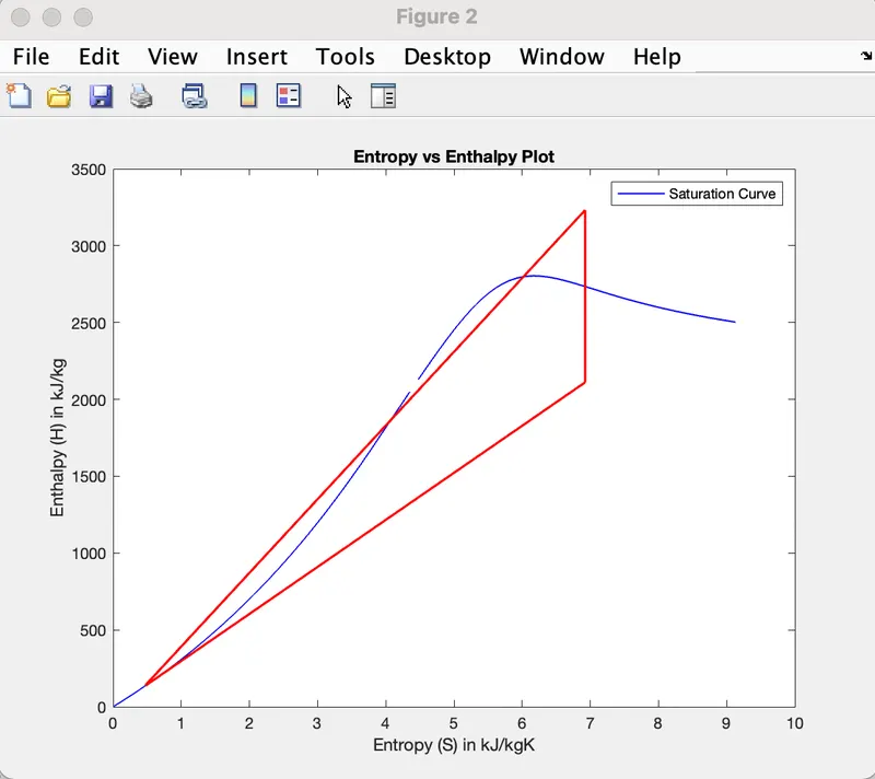
- Plot corresponding T-s and h-s plots for given set of inputs.
- Calculate the Net Work Output and Back Work Ratio.
INTRODUCTION :
The Rankine cycle or Rankine Vapor Cycle is an idealized thermodynamic cycle describing the process by which certain heat engines, such as steam turbines or reciprocating steam engines, allow mechanical work to be extracted from a fluid as it moves between a heat source and a heat sink.
Possible heat sources include combustion of fossil fuels such as coal, natural gas, or oil, renewable fuels like biomass or ethanol, nuclear fission, and concentrated solar power. Common heat sinks include ambient air above or around a facility and bodies of water such as rivers, ponds, and oceans.
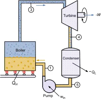
In this mechanism, a fuel is used to produce heat energy to the system via a boiler, converting the working fluid (water) into high pressure steam which then expands through a turbine producing useful work. After passing over the turbine, the fluid is allowed to condense back into a liquid state as waste heat energy is rejected before being returned to the boiler with the help of a pump, completing the cycle.
The various processes involved in the above mentioned figure are as follows :
- Process 1 – 2 – 3 : Isobaric Heat Transfer
In this process, the high pressure liquid enters the boiler from the feed pump. Heat addition process is carried out to first raise its temperature to saturation temperature and further addition of heat leads to evaporation of liquid and then it is converted to steam. - Process 3 – 4 : Isentropic Expansion
This is the reversible expansion process carried out in the turbine in which the steam is expanded and thus resulting in some work output, which may be converted into electricity. The steam is expanded down to the condenser pressure. - Process 4 – 5 : Isobaric Heat Rejection
The vapour – liquid mixture leaving the turbine is subjected to heat rejection process in the condenser so that the steam is condensed to water. - Process 5 – 1 : Isentropic Compression
The pressure of the condensate is raised in the feed pump and is pumped back into the boiler and the cycle is repeated.
GOVERNING EQUATIONS :
- Thermal Efficiency
It is the efficiency of a heat engine measured by the ratio of work done by it to the heat supplied to it.
`eta_(th) = W_("net")/(Q_"in")` `= 1 - Q_(out)/Q_("in")`
Where, `W_"net"` = net work output = `Q_"in" - Q_(out)` - Back Work Ratio
The ratio of the compressor work to the turbine work is called the back-work ratio.
`"BWR" = (h_1 - h_4)/(h_2 - h_3)`
Where `h_1`, `h_2`, `h_3` and `h_4` are the enthalpy values at state point 1, 2, 3 and 4 respectively. - Dryness Fraction
It is used to quantify the amount of water or moisture content within steam.
`x = (s_2 - s_(f2))/(s_(g2)-s_(f2))`
Where, `s_2` = Entropy value at state point 2
`s_(f2)` = Saturated Liquid Entropy at state point 2
`s_(g2)` = Saturated Vapour Entropy at state point 2
PROGRAM CODE AND EXPLANATION :
Program :
% Rankine Cycle Simulator
clear all
close all
clc

% displaying title
fprintf('                RANKINE CYCLE SIMULATOR\n\n')

% printing cycle information
fprintf('Process 1-2 : Isentropic Expansion in the Turbine\n')
fprintf('Process 2-3 : Constant Pressure Heat Rejection by the Condenser\n')
fprintf('Process 3-4 : Isentropic Compression in the Pump\n')
fprintf('Process 4-1 : Constant Pressure Heat Addition by the Boiler\n\n')

% input values for calculating Rankine Cycle data
p1 = input('The value of Pressure at Turbine Inlet (in bar) : ');
T1 = input('The value of Temperature at Turbine Inlet (in °C) : ');
p2 = input('The value of Pressure at Condenser Inlet (in bar) : ');

fprintf('\n                RESULTS\n')

% extracting state variables from Xsteam file
% State Point - 1
h1 = XSteam('h_pT',p1,T1);   % Enthalpy
s1 = XSteam('s_pT',p1,T1);   % Entropy
Ts1 = XSteam('Tsat_p',p1);   % Saturation Temperature
hf1 = XSteam('hL_p',p1);     % Saturated Liquid Enthalpy
hg1 = XSteam('hV_p',p1);     % Saturated Vapour Enthalpy
sf1 = XSteam('sL_p',p1);     % Saturated Liquid Entropy
sg1 = XSteam('sV_p',p1);     % Saturated Vapour Entropy


% State Point - 2
% As it is an Isentropic Expansion Process
s2 = s1;                      % Entropy
sf2 = XSteam('sL_p',p2);      % Saturated Liquid Entropy
sg2 = XSteam('sV_p',p2);      % Saturated Vapour Entropy
x = (s2 - sf2)/(sg2-sf2);     % Dryness Fraction
hf2 = XSteam('hL_p',p2);      % Saturated Liquid Enthalpy
hg2 = XSteam('hV_p',p2);      % Saturated Vapour Enthalpy
h2 = hf2 + x*(hg2 - hf2);     % Enthalpy
T2 = XSteam('T_ph',p2,h2);    % Temperature
Ts2 = XSteam('Tsat_p',p2);    % Saturation Temperature


% State Point - 3
p3 = p2;                      % Constant Pressure Heat Rejection
T3 = T2;                      % Temperature
h3 = XSteam('hL_p',p3);       % Enthalpy
s3 = XSteam('sL_p',p3);       % Entropy

% State Point - 4
s4 = s3;                      % Entropy
p4 = p1;                      % Constant Pressure Heat Addition
h4 = XSteam('h_ps',p4,s4);    % Enthalpy
T4 = XSteam('T_ps',p4,s4);    % Temperature

% Defining Vapour Line Points
T5 = Ts1;
s5 = sf1;
s6 = sg1;
T6 = T5;
h5 = hf1;
h6 = hg1;

% Work done by Turbine
W_turb = h1 - h2;

% Work done by Pump
v3 = XSteam('vL_p',p3);       % Saturated Liquid Volume
W_pump = v3*(p4-p3)*100;

% Net Work Done
W_net = W_turb - W_pump;

% Heat Input into the system
Q_in = h1 - h4;

% Heat Output from the system
Q_out = h2 - h3;

% Thermal Efficiency of Rankine Cycle
efficiency = (W_net/Q_in)*100;

% Steam Rate
steam_rate = 3600/W_net;

% Back Work Ratio
BWR = W_pump/W_turb;

% Plotting the Saturation Curve
% Defining Temperature Range
T = linspace(1,375,1000);

for i = 1:length(T)
    sf(i) = XSteam('sL_T',T(i));
    sg(i) = XSteam('sV_T',T(i));
    hf(i) = XSteam('hL_T',T(i));
    hg(i) = XSteam('hV_T',T(i));
end


% Plotting the T - s diagram
figure(1)
hold on
plot(sf,T,'Color','b','LineWidth',1)
plot(sg,T,'Color','b','LineWidth',1)
plot([s1 s2],[T1 T2],'Color','r','LineWidth',1.5)
plot([s2 s3],[T2 T3],'Color','r','LineWidth',1.5)
plot([s3 s4],[T3 T4],'Color','r','LineWidth',1.5)

sc4 = linspace(s4,s5,1000);
for j = 1:length(sc4)
    Tc4(j) = XSteam('T_ps',p4,sc4(j));
end

plot([sc4 s5],[Tc4 T5],'Color','r','LineWidth',1.5)
plot([s5 s6],[T5 T6],'Color','r','LineWidth',1.5)
plot([s6 s1],[T6 T1],'Color','r','LineWidth',1.5)
title('Entropy vs Temperature Plot')
xlabel('Entropy (S) in kJ/kgK')
ylabel('Temperature (T) in °C')
legend('Saturation Curve')


% Plotting h - s diagram
figure(2)
plot(sf,hf,'Color','b','LineWidth',1)
hold on
plot(sg,hg,'Color','b','LineWidth',1)
plot([s1 s2],[h1 h2],'Color','r','LineWidth',1.5)
plot([s2 s3],[h2 h3],'Color','r','LineWidth',1.5)
plot([s3 s4],[h3 h4],'Color','r','LineWidth',1.5)
plot([s4 s1],[h4 h1],'Color','r','LineWidth',1.5)
title('Entropy vs Enthalpy Plot')
xlabel('Entropy (S) in kJ/kgK')
ylabel('Enthalpy (H) in kJ/kg')
legend('Saturation Curve')

% printing results in command window
fprintf('At state point 1 : \n')
fprintf('P1 is : %.0f Bar\n',p1)
fprintf('T1 is : %.0f °C\n',T1)
fprintf('H1 is : %.2f kJ/kg\n',h1)
fprintf('S1 is : %.2f kJ/kgK\n\n',s1)

fprintf('At state point 2 : \n')
fprintf('P2 is : %.2f Bar\n',p2)
fprintf('T2 is : %.2f °C\n',T2)
fprintf('H2 is : %.2f kJ/kg\n',h2)
fprintf('S2 is : %.2f kJ/kgK\n\n',s2)

fprintf('At state point 3 : \n')
fprintf('P3 is : %.2f Bar\n',p3)
fprintf('T3 is : %.2f °C\n',T3)
fprintf('H3 is : %.2f kJ/kg\n',h3)
fprintf('S3 is : %.2f kJ/kgK\n\n',s3)

fprintf('At state point 4 : \n')
fprintf('P4 is : %.2f Bar\n',p4)
fprintf('T4 is : %.2f °C\n',T4)
fprintf('H4 is : %.2f kJ/kg\n',h4)
fprintf('S4 is : %.2f kJ/kgK\n\n',s4)

fprintf('Turbine Work : %.2f kJ/kg\n',W_turb)
fprintf('Pump Work    : %.2f kJ/kg\n',W_pump)
fprintf('Net Work     : %.2f kJ/kg\n',W_net)
fprintf('Efficiency   : %.2f percent\n',efficiency)
fprintf('Steam Rate   : %.2f kg/kWh\n',steam_rate)
fprintf('Back Work Ratio : %.4f \n',BWR)
Explanation :
- We begin the program by using the clear all, close all and clc commands to clear up the workspace as well as the command window.
- We use the ‘XSteam’ data file to extract the required data of Enthalpy, Entropy, Temperatures and values of saturated liquid and vapor as well.
Example : The command XSteam(‘h_pT’, p , T) extracts the Enthalpy value as a function of Pressure (p) and Temperature (T).
- The next step involves defining the input conditions as given in the problem, by using the ‘input’ function, which displays the text in prompt and waits for user to input a value.
We define the input conditions of pressure at turbine inlet (p1), temperature at turbine inlet (T1) and the pressure at the condenser inlet (p2), at this stage.
- In the next step, with the help of the input data and the values extracted from the XSteam table, we calculate the values of
- Enthalpy ( h )
- Entropy ( s )
- Saturated Liquid Enthalpy ( `h_f` )
- Saturated Vapor Enthalpy ( `h_g` )
- Saturated Liquid Entropy ( `s_f` )
- Saturated Vapor Entropy ( `s_g` )
- Saturation Temperature ( `T_(sat)` )
- Process Temperature ( T )
- Dryness Fraction ( x )
These values are calculated for all 4 state points of the process, as and when required, by using the appropriate formulas and thermodynamic relations along with the data generated from the XSteam tables.
- With the help of the above extracted values, we then calculate the values of
- Work done by the Turbine ( `W_(turb)`)
- Work done by the pump ( `W_(pump)` )
- Net Work done ( `W_("net")` )
- Heat Input into the System ( `Q_("in")` )
- Heat Output from the System ( `Q_(out)` )
- Thermal Efficiency of Rankine Cycle ( `eta` )
- Steam Rate
- Back Work Ratio ( BWR )
- In the next step, we plot the T-s diagram along with the saturation line. In order to do so, we first define a temperature range from 1 to 375 degree celcius with 1000 values inbetween it, using the linspace
As the connecting line from process 4 – 5 is a curve, we use the for loop function to plot the points along the temperature range to obtain the curve. A plot of the Saturation Curve is obtained by plotting the Saturated Entropy of liquid and vapor (`s_f` and `s_g`) against Temperature (T).
Thereby, we plot the Entropy (s) on the x-axis and Temperature (T) on the y-axis to get the required T-s plot of the processes.
- Similarly, we obtain the H-S plot of the processes by plotting Entropy (s) on the x-axis and Enthalpy (h) on the y-axis for the entire range of values. The saturation curve for the same is obtained by plotting the Saturated Entropies of liquid and vapor (`s_f` and `s_g`) against Saturated Enthalpies of liquid and vapor (`h_f` and `h_g)`.
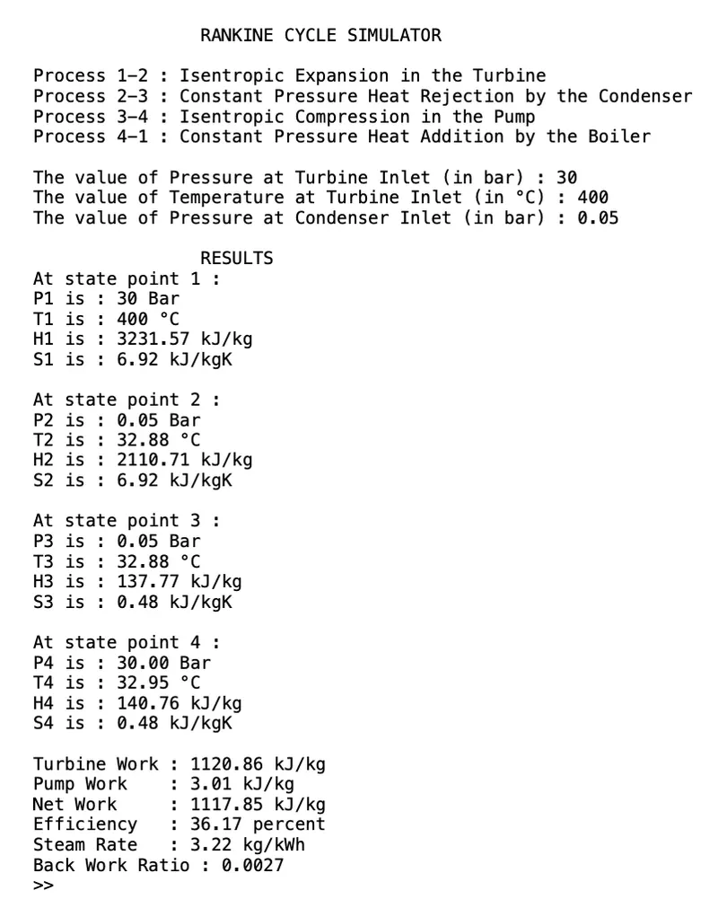
- Finally, we use the ‘fprintf’ command to print all the obtained and calculated results and thereby displaying the desired results on screen.
OUTPUTS :
1. T-s plot :
2. H-s plot :
3. Results in command window :
CONCLUSION :
- The program to simulate a Rankine Cycle has been successfully written.
- The state points for all states of the process have been calculated based on the inputs provided and the values of which are displayed in the command window.
- The corresponding T-s and H-s diagrams for the cycle have been plotted with reference to the variables calculated.
- From the provided input values, we get the corresponding outputs as follows :
i. Net Work = 1117.85 kJ/kg
ii. Thermal Efficiency = 36.17 %
iii. Back Work Ratio = 0.0027
REFERENCES :
https://energyeducation.ca/encyclopedia/Rankine_cycle
https://en.wikipedia.org/wiki/Rankine_cycle