Week 9 - Parametric study on Gate valve.
AIM :
To perform a parametric study on the gate valve simulation.
OBJECTIVES :
- Perform a parametric study on the gate valve, by setting the opening from 10% to 80%.
- Obtain the mass flow rates at the outlet for each design point and discuss the results.
- Calculate the flow coefficient and flow factor for each opening and plot the graph.
INTRODUCTION :
A gate valve is an on-off valve that works by inserting a rectangular gate or wedge into the flow of the fluid. It is generally used to completely shut off fluid flow rather than for flow regulation. When fully open, the typical gate valve has no obstruction in the flow path, resulting in very low flow resistance.
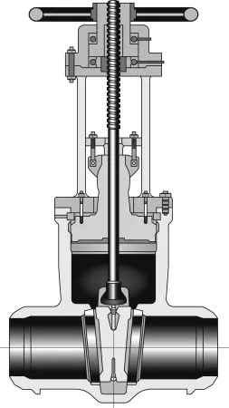
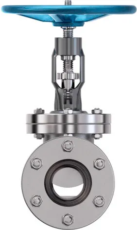
A gate valve consists of a valve body, seat and disc, a spindle, gland and a wheel for operating the valve. The seat and the gate together perform the function of shutting off the flow of fluid.
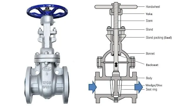
How does a gate valve operate?
A gate valve operates similar to other valves. To open the valve, turn the handwheel, which moves the gate up or down on the stem via the threads. A gate valve requires more than one 360° turn to open or close the valve fully. When the gate is lifted up, it opens the inlet to the outlet allowing an unobstructed passageway for the media to flow. When the gate is lowered, it closes and blocks the media flow.
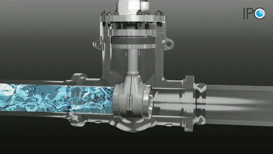
Gate valves are available in different types, such as slab, expanding and wedge.
FLOW CO-EFFICIENT :
The flow coefficient of a device is a relative measure of its efficiency at allowing fluid flow. It describes the relationship between the pressure drop across an orifice valve or other assembly and the corresponding flow rate.
Mathematically the flow coefficient `C_"v"` (or flow-capacity rating of valve) can be expressed as,
`C_"v" = Q * sqrt ((SG) / (DeltaP)`
Where,
`Q` = Rate of flow (expressed in US gallons per minute)
`SG` = Specific gravity of the fluid (for water = 1)
`DeltaP` = Pressure drop across the valve (expressed in psi).
FLOW FACTOR :
The metric equivalent flow factor (`K_"v"`) is calculated using metric units,
`K_"v" = Q *sqrt ((SG) / (DeltaP))`
Where,
`K_"v"` = Flow factor (expressed in m3·h−1)
`Q` = Flowrate (expressed in cubic metres per hour m3·h−1),
`SG` = Specific gravity of the fluid (for water = 1),
`DeltaP` = Differential pressure across the device (expressed in bar).
`K_"v"` can be calculated from `C_"v"` using the equation,
`K_"v" = 0.865 * C_"v"`
PARAMETRIC STUDY PROCEDURE :
The workflow of the simulation is carried out in 6 steps. As we are parameterizing certain dimensions of the study, we get an additional parameter step.
- Geometry
- Meshing
- Setup
- Solution
- Results
- Parameters
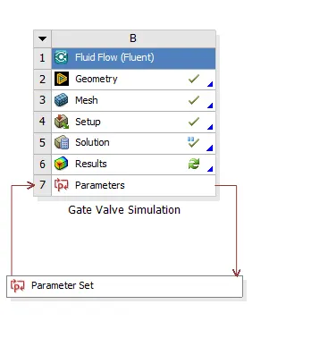
1. GEOMETRY
In this step, we first import the step file geometry into the ANSYS SpaceClaim software as shown.
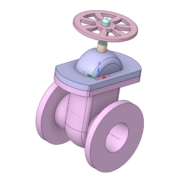
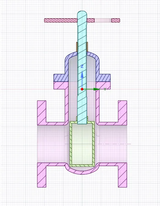
The various components of the gate valve geometry is as follows.
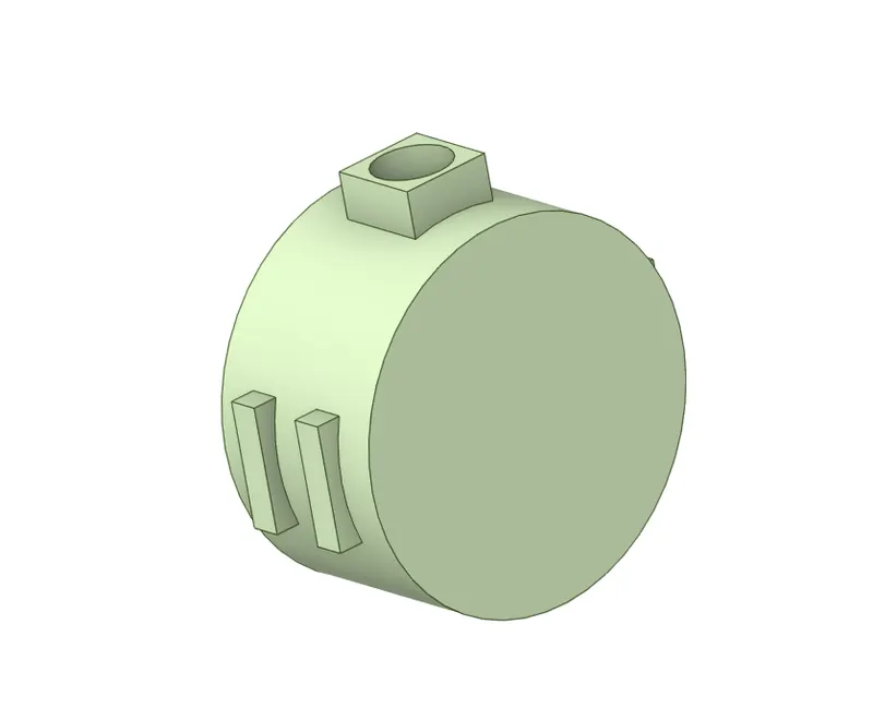
i.) Gate Disc
The gate disc is the part of the valve that regulates the flow of water through it. When it is in a completely closed position, it completely shuts off flow and when it is in a fully open position, it provides full flow in a pipeline.
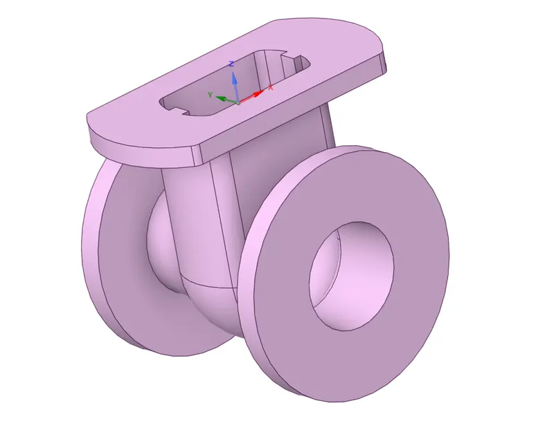
ii.) Bottom
The valve bottom is the main pressure-retaining part, that also holds other parts such as disc and spindle. This also provides passage to flow from the valve to its end connection, which is the piping.
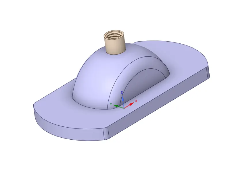
iii.) Bonnet
The purpose of the bonnet is to provide coverage for the internal components of a gate valve. The bonnet of a gate valve contains moving parts and typically attaches to the body of the valve using bolts or screws to form a leak-proof seal.
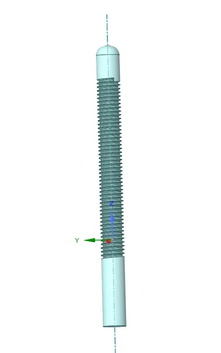
iv.) Spindle
The purpose of the spindle in a gate valve is to raise or lower the gate. Users can complete this task by spinning the threaded spindle manually or controlling it using an actuator.
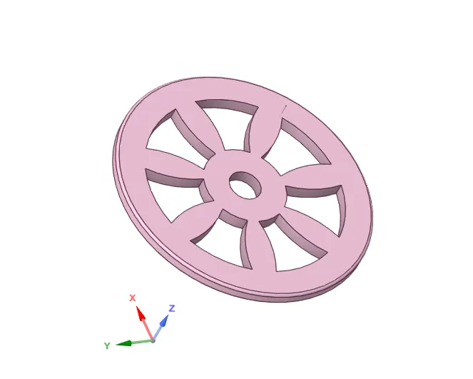
v.) Hand Wheel
The handwheel is used to manually actuate the movement of the gate.
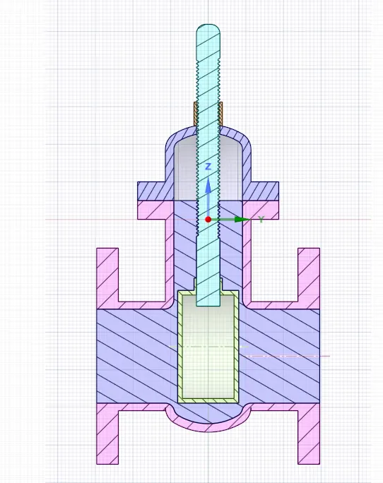
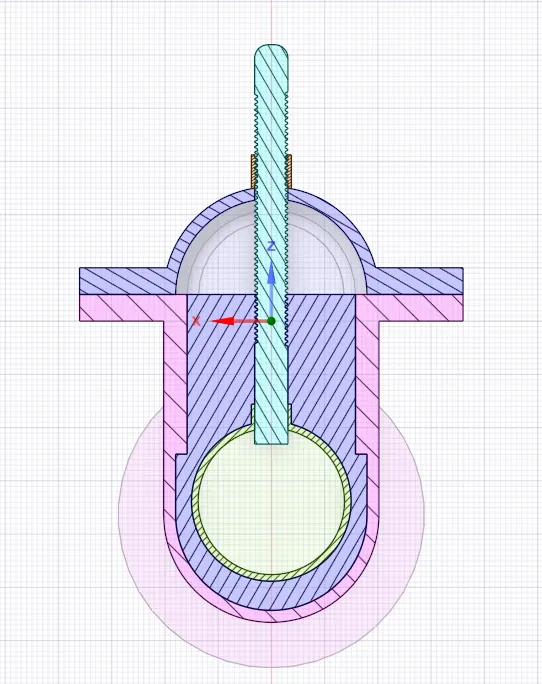
The cross – sectional view of the geometry is represented as follows.
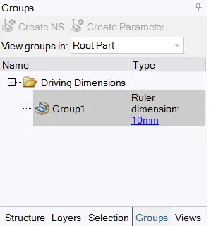
The next step involves giving an initial level of lift for the gate, which permits the flow of water through it. We initially raise the gate up by 10 mm. We do this by using the ‘move’ command.
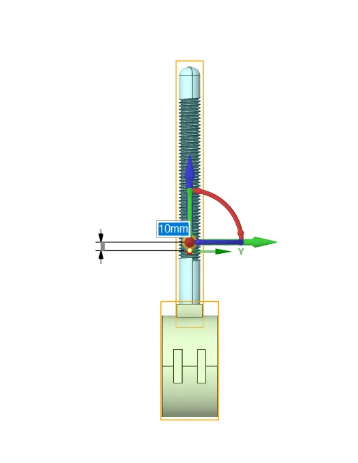
We parameterize the initial lift such that we can vary this dimension and obtain the outputs for different values of gate disc lift.
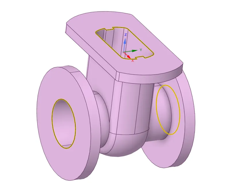
The next step in geometry preparation is performing volume extraction, where we extract the fluid volume of the geometry. We select the inlet, outlet and the region where the fluid is contained, which is hidden under the bonnet as shown.
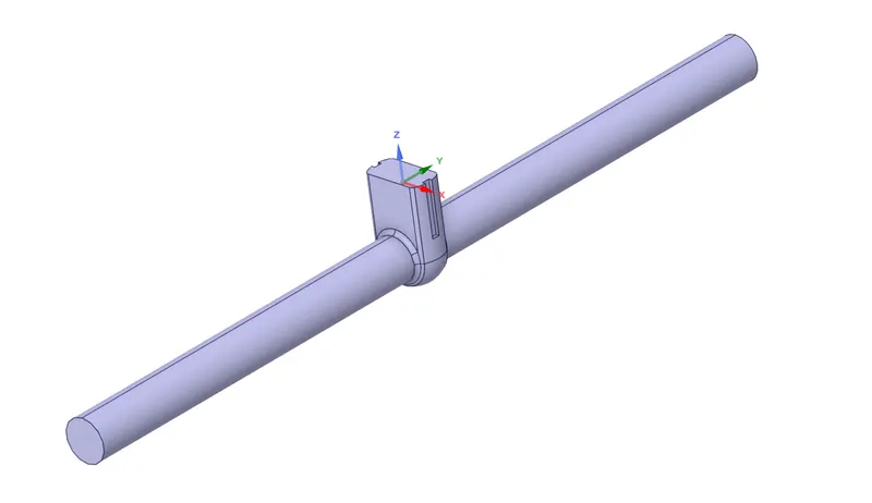
After obtaining the fluid volume extraction, we extend the fluid flow regions of the inlet and outlet, using the ‘pull’ function. We extend it to a length of 800 mm.
2. MESHING
Before generating the mesh for the geometry, we first create the named selections for the inlet and outlet of the valve as shown below.
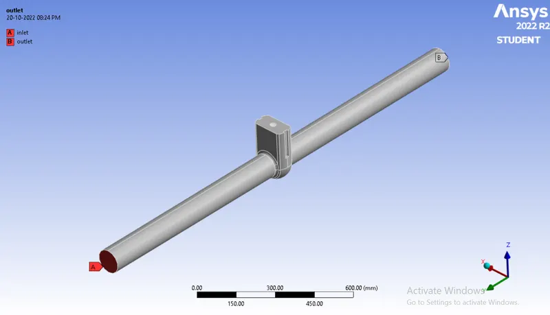
Next, we generate the base meshing of default mesh size for the geometry. We obtain the mesh model as follows.
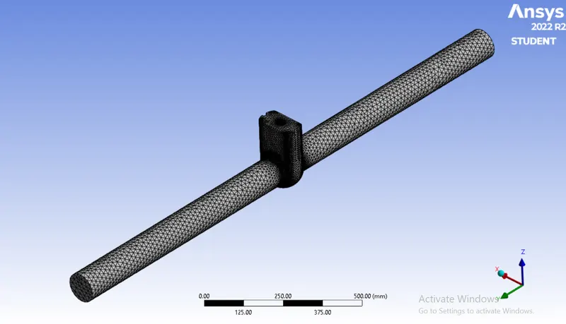
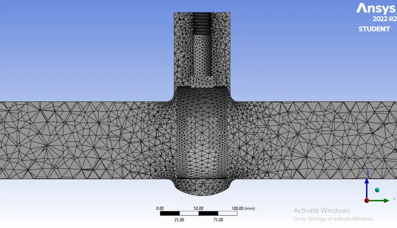
3. SETUP
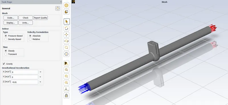
We setup the general parameters for the simulation as follows.
- We use a pressure – based steady state solver with absolute velocity formulation for this simulation.
- We enable gravity on the negative z – axis for a value of – 9.81 m/s.
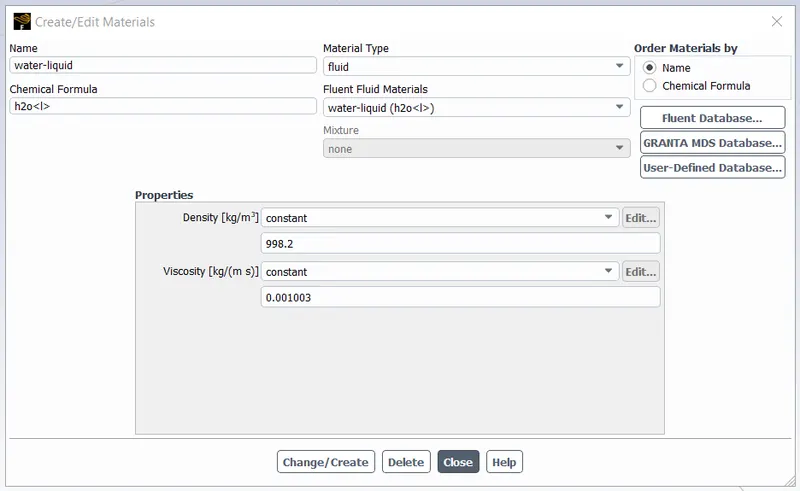
We consider the working fluid flowing through the gate valve section to be water at its standard properties.
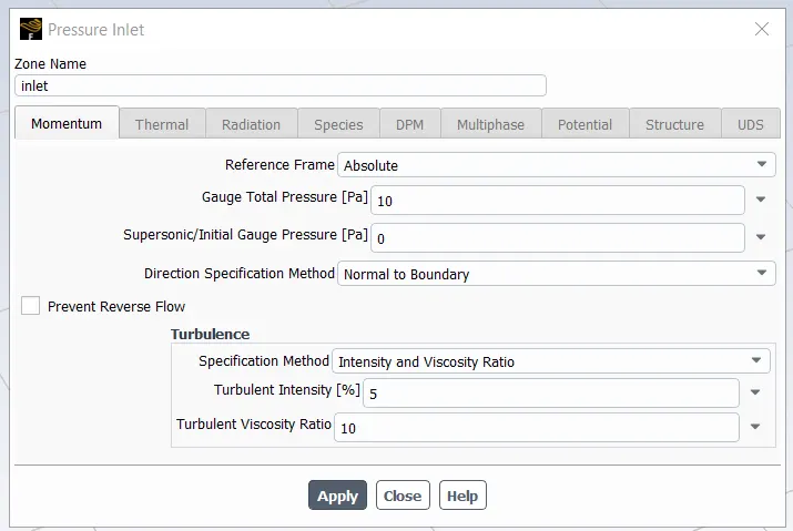
We provide the inlet boundary conditions as a pressure inlet with a total gauge pressure of 10 Pa. The outlet is considered as a pressure outlet a 0 Pa gauge pressure.
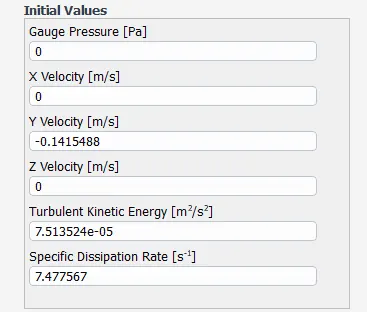
If we standard initialize the simulation, we can calculate the value of initial velocity at the inlet as 0.1415 m/s.
From this initial velocity value and previously defined values of density of water and inlet diameter, we calculate the Reynold’s number of the flow.
i.) Density of Water `rho` `=` `998.2` `kg`/`m^3`
ii.) Inlet Diameter `D` `=` `0.1` `m`
iii.) Initial Velocity at Inlet `v` `=` `0.1415` `m`/`s`
iv.) Dynamic Viscosity of Water `mu` `=` `0.001003` `kg`/`m*s`
We know, the Reynold’s number is given by,
`R_e = (rho * v * D) / mu`
`R_e = (998.2 xx 0.1415 xx 0.1)/0.001`
`R_e` = 14124.53
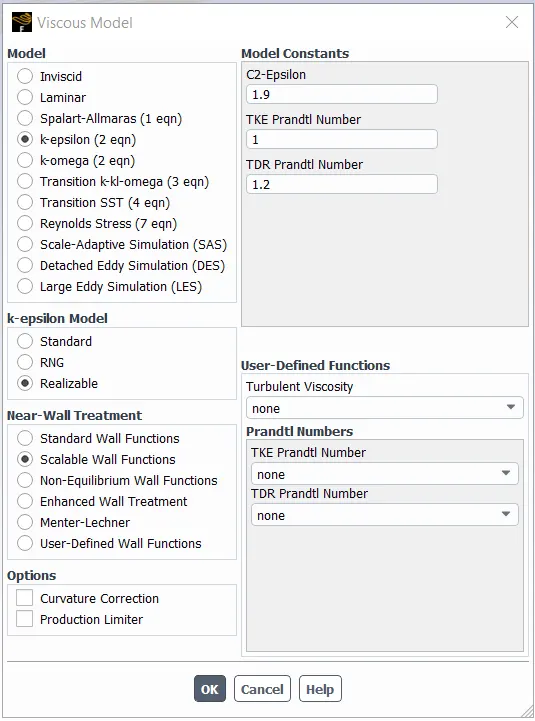
From the Reynold’s number value obtained, we can infer that the fluid flow is turbulent in nature, as the `R_e` value is greater than `3000`. Thereby, we use the realizable k – epsilon turbulence model with scalable wall functions for this simulation.
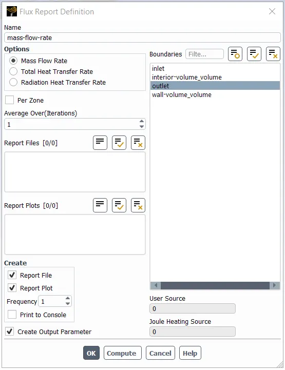
In the next step, we define the flux report to evaluate the mass flow rate at the outlet. We create an output parameter of the same, so as to include the calculated values in our parametric study table.
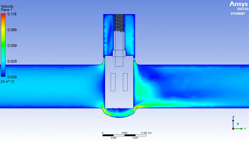
Finally, we standard initialize the simulation and setup a contour plot to visualize the velocity of fluid flow through the gate opening. We also setup a solution animation for the same.
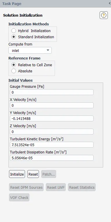
We run the solution for 200 iterations to obtain the output plots and contours.
For the parametric study of the simulation, we are going to consider 8 different levels of disc lift, i.e., from 10 mm – 80 mm. We simulate each case study to observe the effects of lift on the fluid flow and obtain the following results.
Case – 1 : 10 mm Disc Lift
In this case study, we raise the gate disc up by 10 mm with respect to its initial position and thereby leading to an increase in mass flow rate across the outlet, as more fluid passes through the gate opening.
The cross section of the lifted gate disc is represented as,
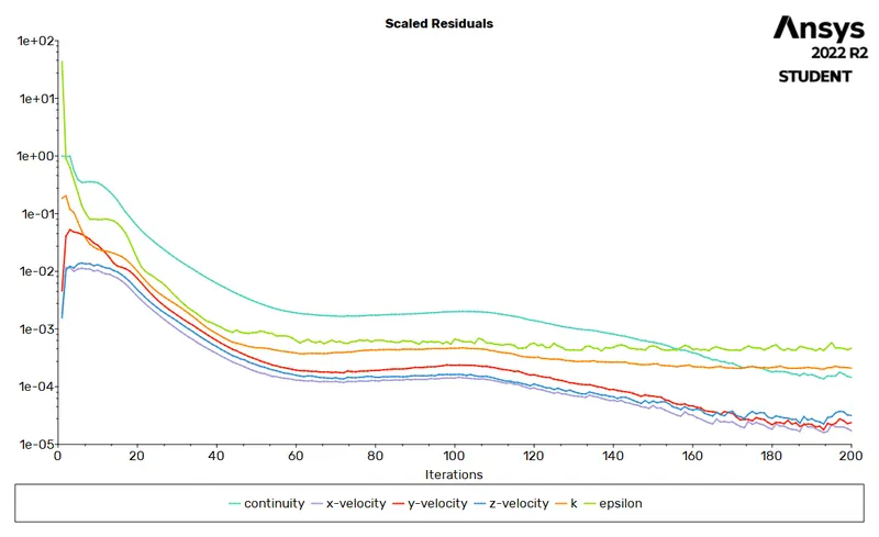
By running the simulation for 200 iterations, we obtain the following outputs.
Residuals Plot :
Mass Flow Rate :
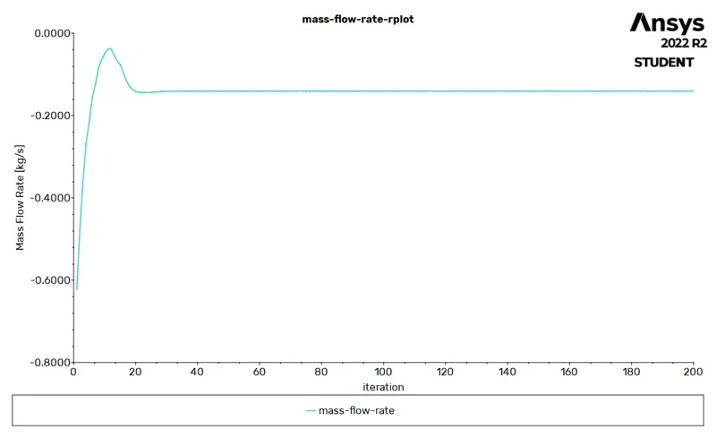
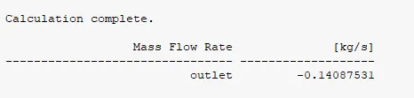
The negative sign of the mass flow rate value signifies that the mass is exiting the system.
Velocity Contour :
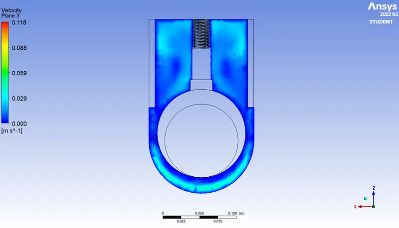
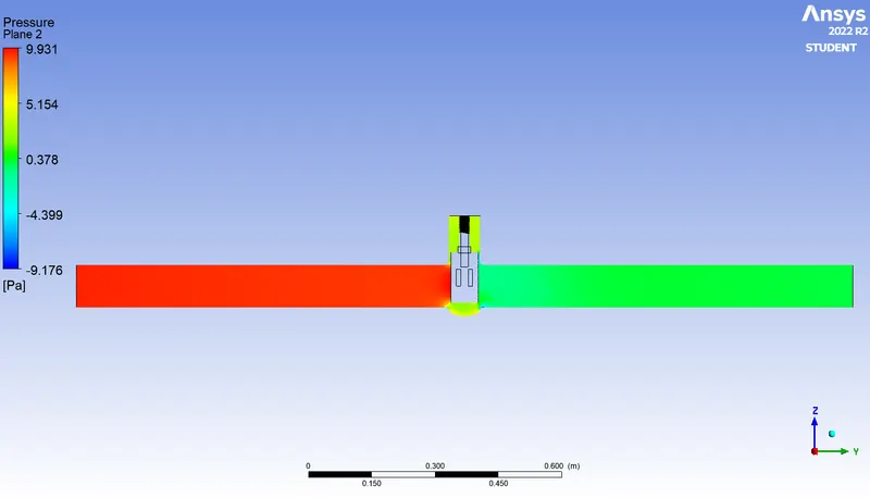
Pressure Contour :
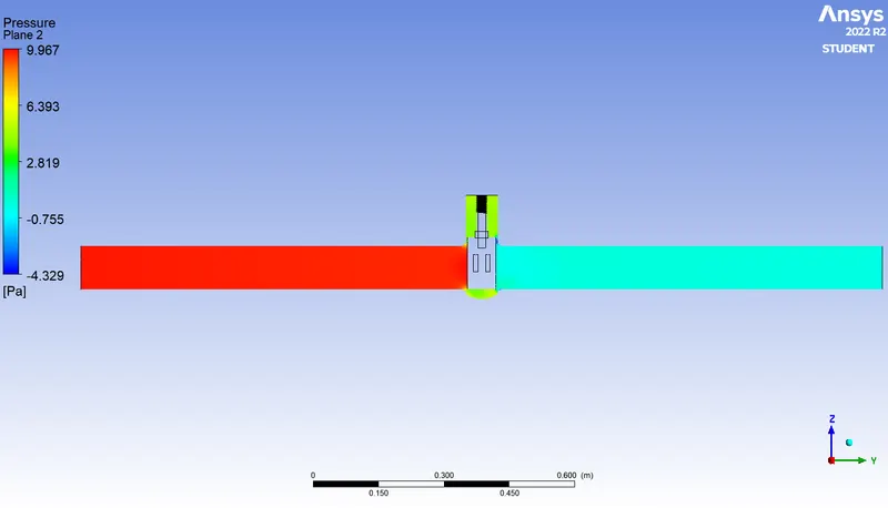
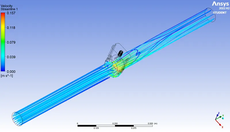
Velocity Streamline Contour :
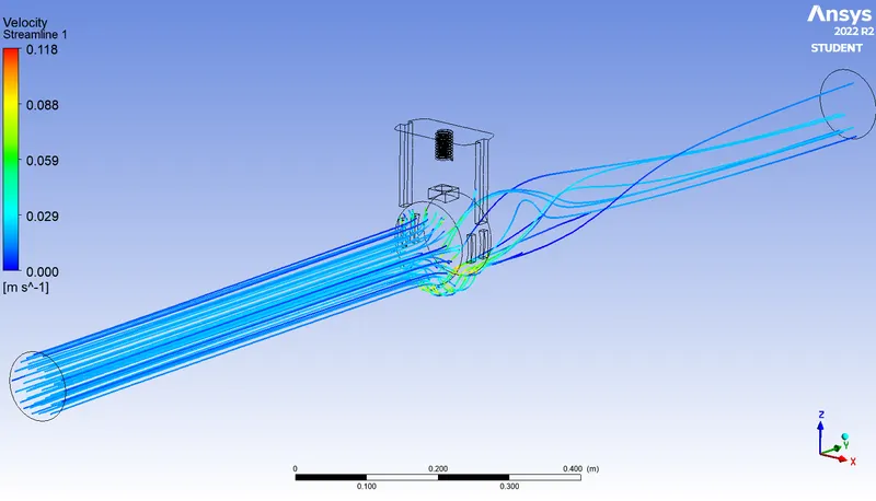
Flow Co-Efficient and Flow Factor :
As we know, flow co-efficient is mathematically expressed as,
`C_"v" = Q * sqrt ((SG) / (DeltaP)`
In this particular case study,
`Q` = Mass Flow Rate = `-0.1408` `kg`/`sec`
= `-2.2317` `gallons`/`min`
`SG` = Specific Gravity of Water = `1`
`DeltaP` = Pressure Drop = `10` `Pa`
= `0.00145` `"psi"`
Therefore,
`C_"v" = 2.2317xx sqrt (1 / 0.00145)`
Flow Co-efficient `C_"v"` = 58.607
Similarly,
Flow Factor `K_"v" = 0.865 * C_"v"`
`K_"v" = 0.865 xx 58.607`
`therefore` `K_"v"` = 50.6953
Case – 2 : 20 mm Disc Lift
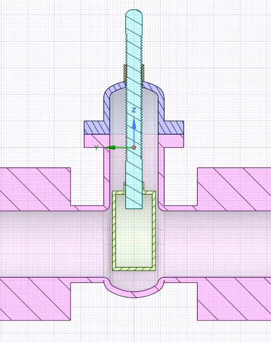
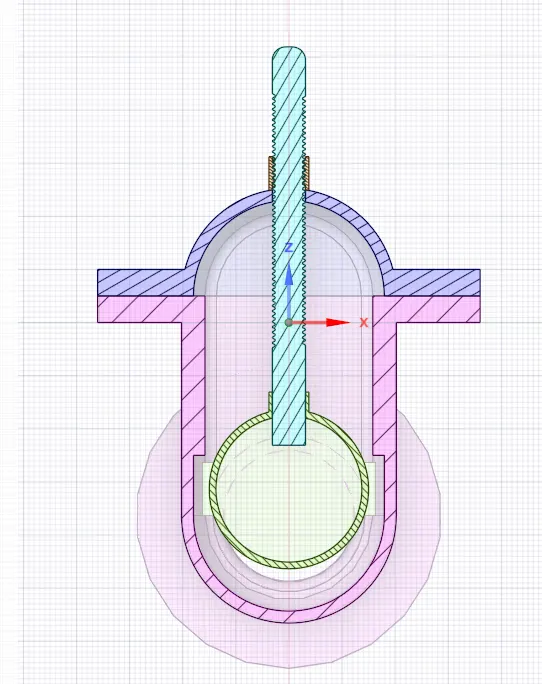
In this case study, we raise the gate disc up by 20 mm with respect to its initial position and we study the effects of this change on the mass flow rate.
The cross section of the lifted gate disc is represented as,
By running the simulation for 200 iterations, we obtain the following outputs.
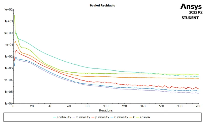
Residuals Plot :
Mass Flow Rate :
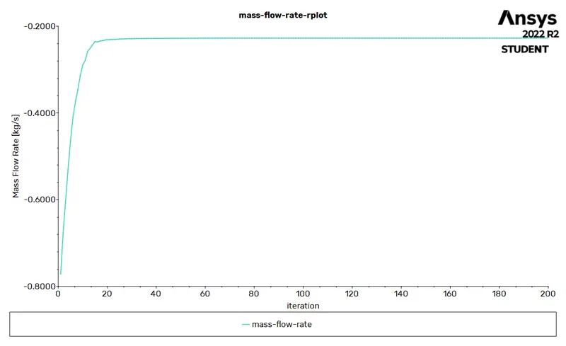
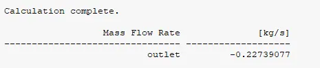
The negative sign of the mass flow rate value signifies that the mass is exiting the system.
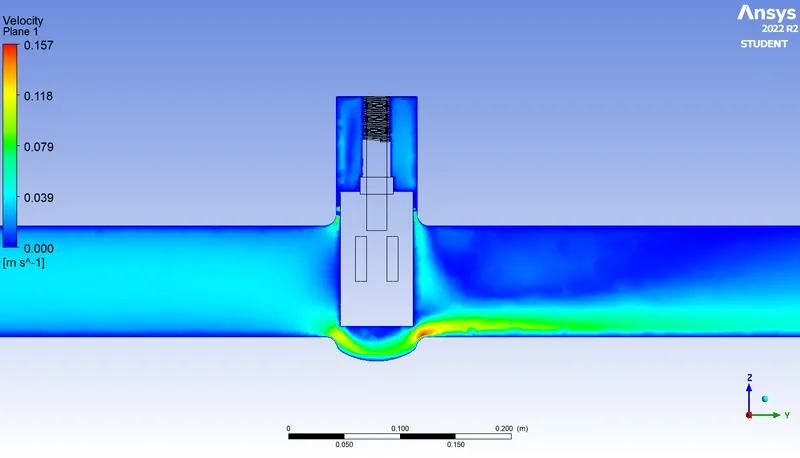
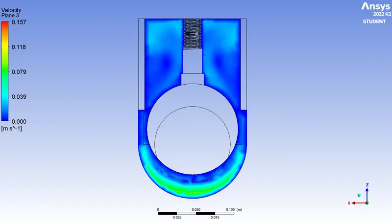
Velocity Contour :
Pressure Contour :
Velocity Streamline Contour :
Flow Co-Efficient and Flow Factor :
In this particular case study,
`Q` = Mass Flow Rate = `-3.6028` `gallons`/`min`
`SG` = Specific Gravity of Water = `1`
`DeltaP` = Pressure Drop = `0.00145` `"psi"`
Therefore,
`C_"v" = 3.6028 xx sqrt (1 / 0.00145)`
Flow Co-efficient `C_"v"` = 94.6141
Similarly,
`K_"v" = 0.865 * C_"v"`
`K_"v" = 0.865 xx 94.6141`
`therefore` Flow Factor `K_"v"` = 81.8412
Case – 3 : 30 mm Disc Lift
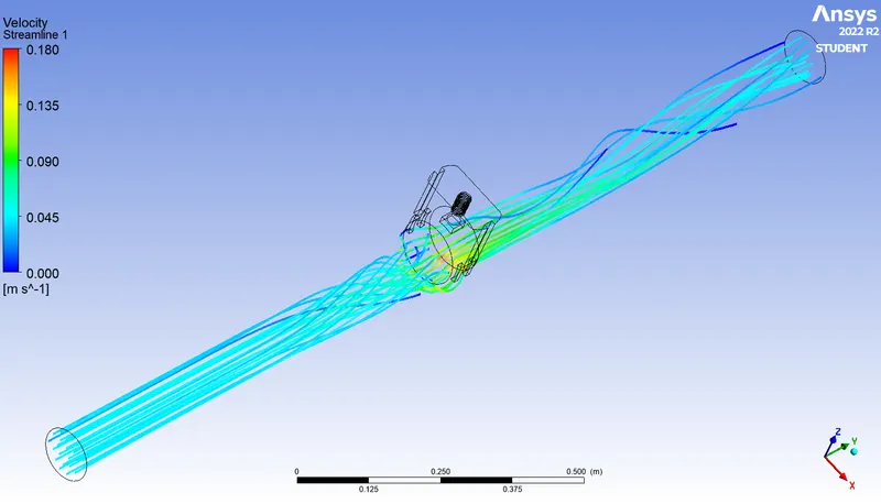
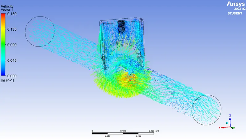
In this case study, we raise the gate disc up by 30 mm with respect to its initial position and we study the effects of this change on the mass flow rate.
The cross section of the lifted gate disc is represented as,
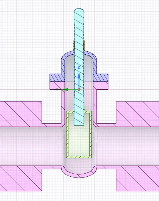
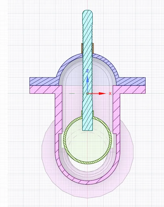
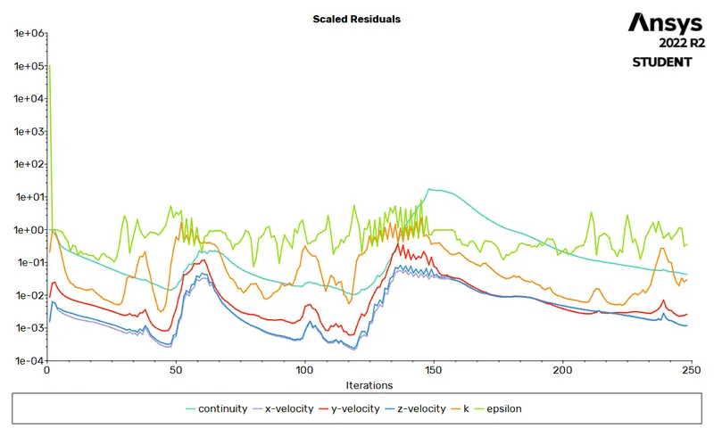
By running the simulation for 250 iterations, we obtain the following outputs.
Residuals Plot :
Mass Flow Rate :
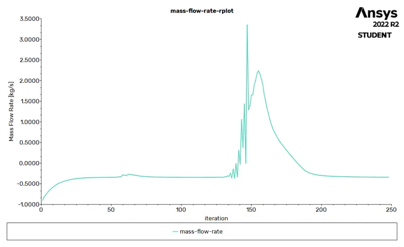
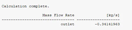
The negative sign of the mass flow rate value signifies that the mass is exiting the system.
Velocity Contour :
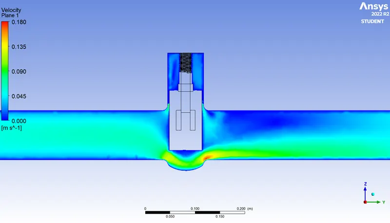
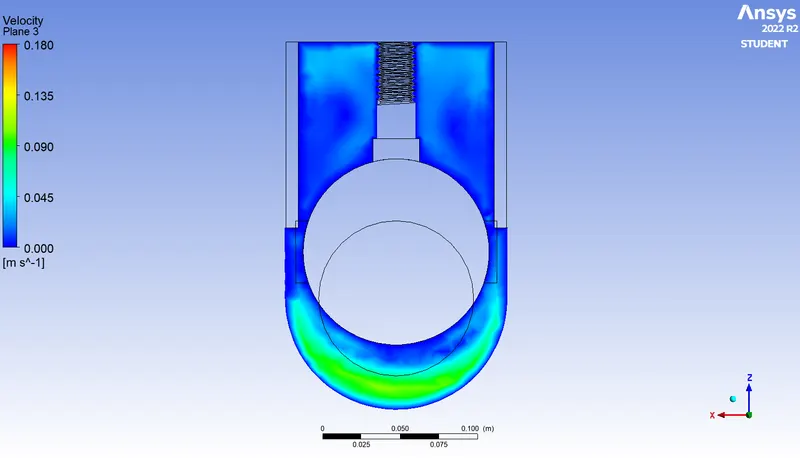
Pressure Contour :
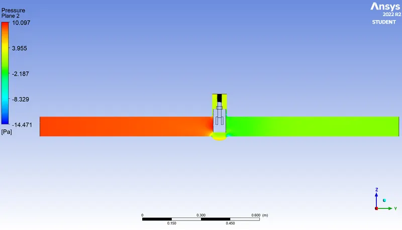
Velocity Streamline Contour :
Vector Plot :
Flow Co-Efficient and Flow Factor :
In this particular case study,
`Q` = `-5.4113` `gallons`/`min`
`SG` = `1`
`DeltaP` = `0.00145` `"psi"`
Therefore,
`C_"v" = 5.4113 xx sqrt (1 / 0.00145)`
Flow Co-efficient `C_"v"` = 142.1077
Similarly,
`K_"v" = 0.865 * C_"v"`
`K_"v" = 0.865 xx 142.1077`
`therefore` Flow Factor `K_"v"` = 122.9231
Case – 4 : 40 mm Disc Lift
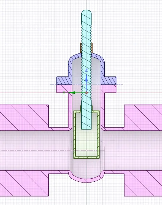
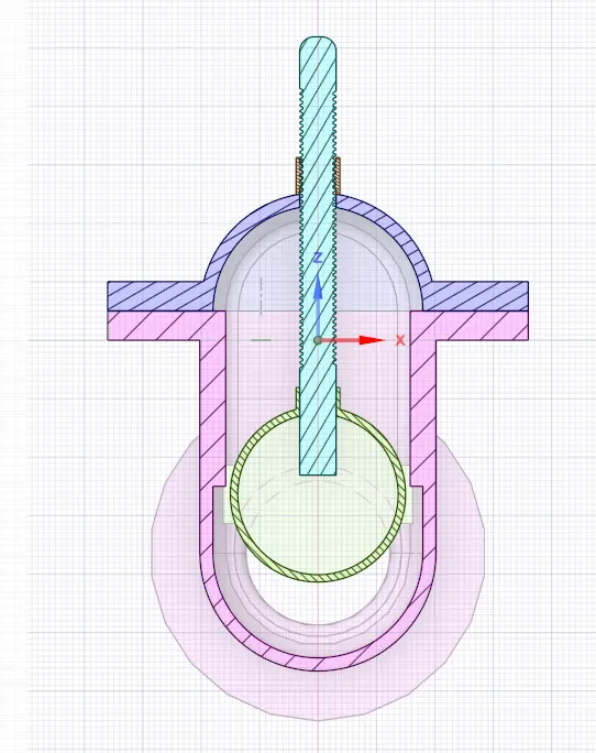
In this case study, we raise the gate disc up by 40 mm with respect to its initial position and we study the effects of this change on the mass flow rate.
The cross section of the lifted gate disc is represented as,
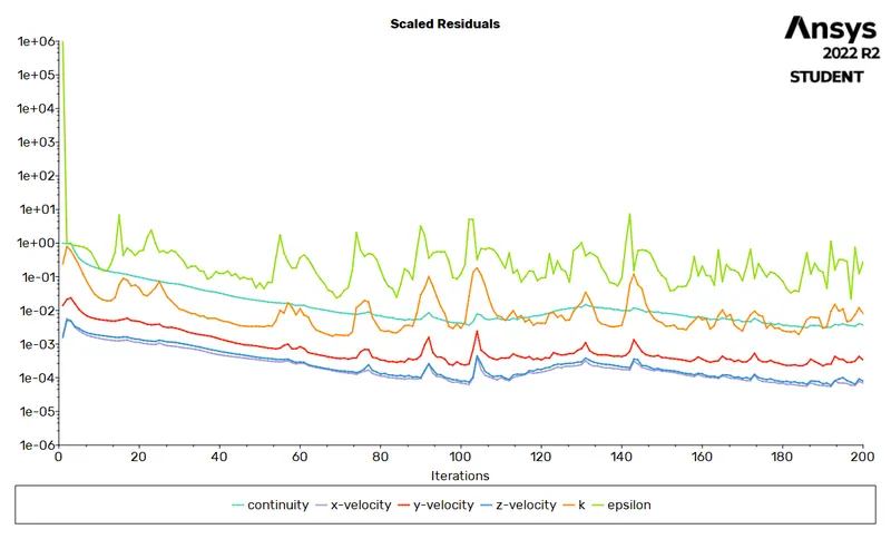
By running the simulation for 200 iterations, we obtain the following outputs.
Residuals Plot :
Mass Flow Rate :
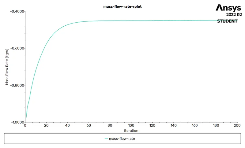
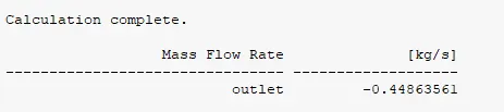
The negative sign of the mass flow rate value signifies that the mass is exiting the system.
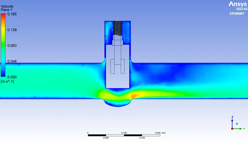
Velocity Contour :
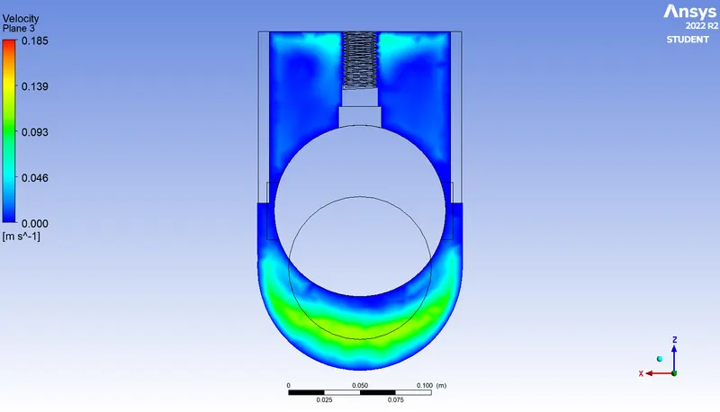
Pressure Contour :
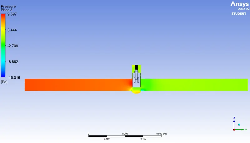
Velocity Streamline Contour :
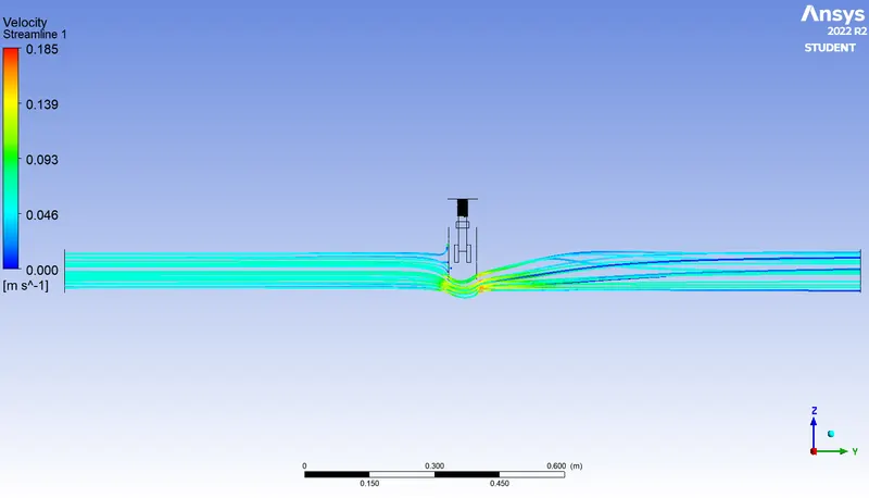
Flow Co-Efficient and Flow Factor :
In this particular case study,
`Q` = `-7.1105` `gallons`/`min`
`SG` = `1`
`DeltaP` = `0.00145` `"psi"`
Therefore,
`C_"v" = 7.1105 xx sqrt (1 / 0.00145)`
Flow Co-efficient `C_"v"` = 186.7308
Similarly,
`K_"v" = 0.865 * C_"v"`
`K_"v" = 0.865 xx 186.7308`
`therefore` Flow Factor `K_"v"` = 161.5222
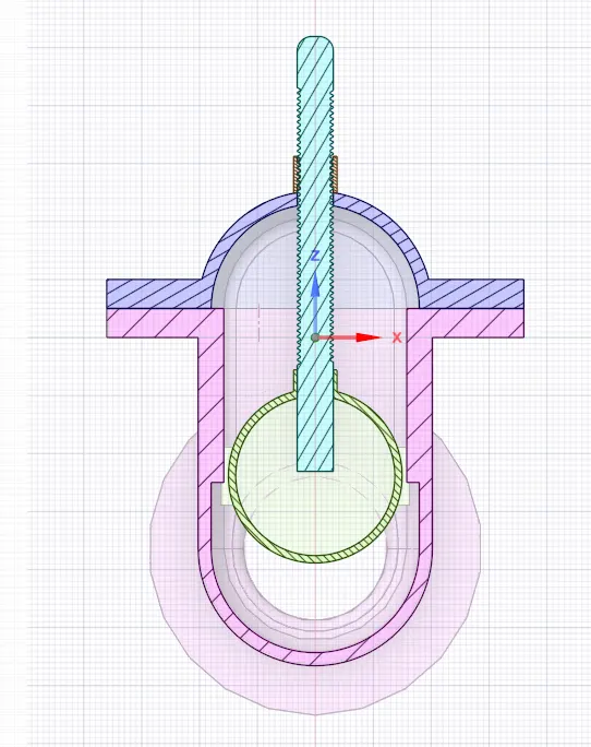
Case – 5 : 50 mm Disc Lift
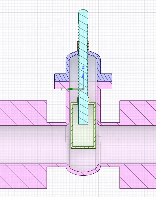
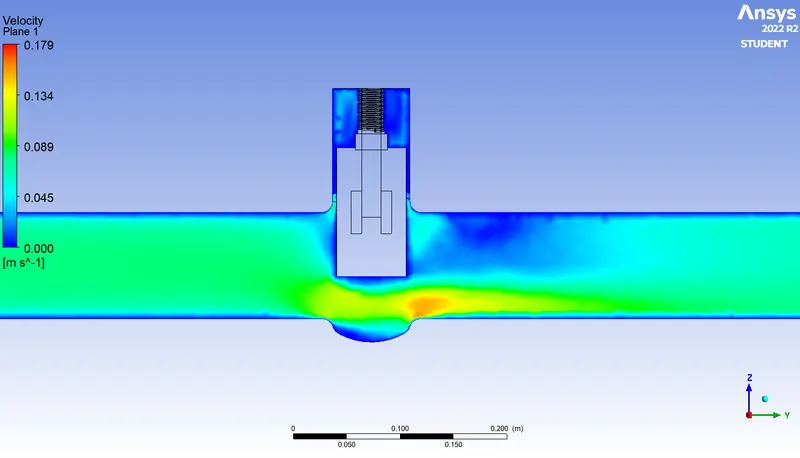
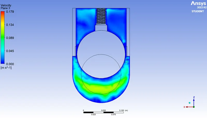
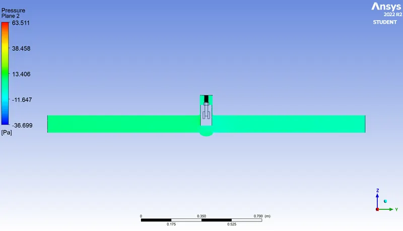
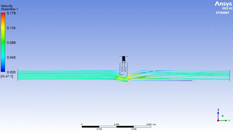
In this case study, we raise the gate disc up by 50 mm with respect to its initial position and we study the effects of this change on the mass flow rate.
The cross section of the lifted gate disc is represented as,
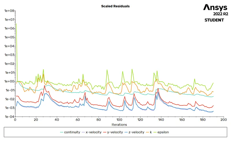
By running the simulation for 200 iterations, we obtain the following outputs.
Residuals Plot :
Mass Flow Rate :
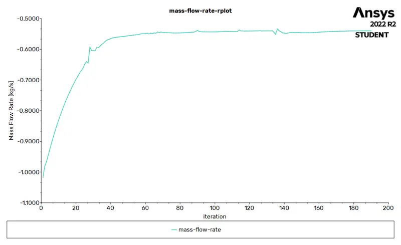
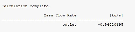
The negative sign of the mass flow rate value signifies that the mass is exiting the system.
Velocity Contour :
Pressure Contour :
Velocity Streamline Contour :
Flow Co-Efficient and Flow Factor :
In this particular case study,
`Q` = `-8.5623` `gallons`/`min`
`SG` = `1`
`DeltaP` = `0.00145` `"psi"`
Therefore,
`C_"v" = 8.5623 xx sqrt (1 / 0.00145)`
Flow Co-efficient `C_"v"` = 224.8570
Similarly,
`K_"v" = 0.865 * C_"v"`
`K_"v" = 0.865 xx 224.8570`
`therefore` Flow Factor `K_"v"` = 194.5013
Case – 6 : 60 mm Disc Lift
In this case study, we raise the gate disc up by 60 mm with respect to its initial position and we study the effects of this change on the mass flow rate.
The cross section of the lifted gate disc is represented as,
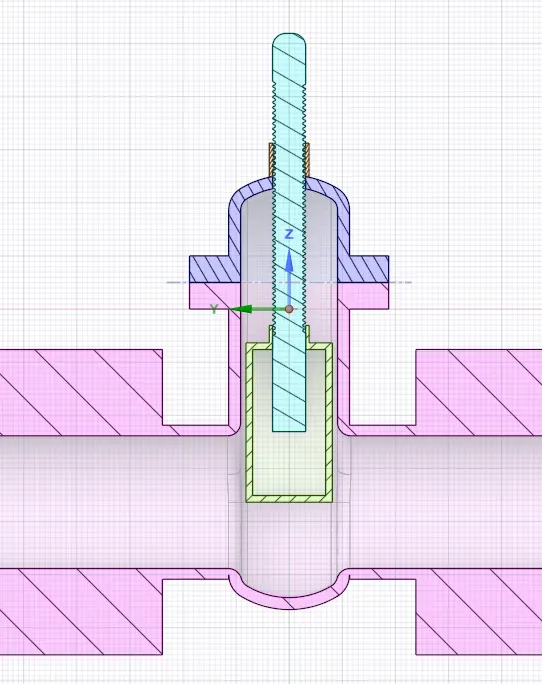
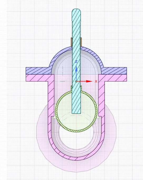
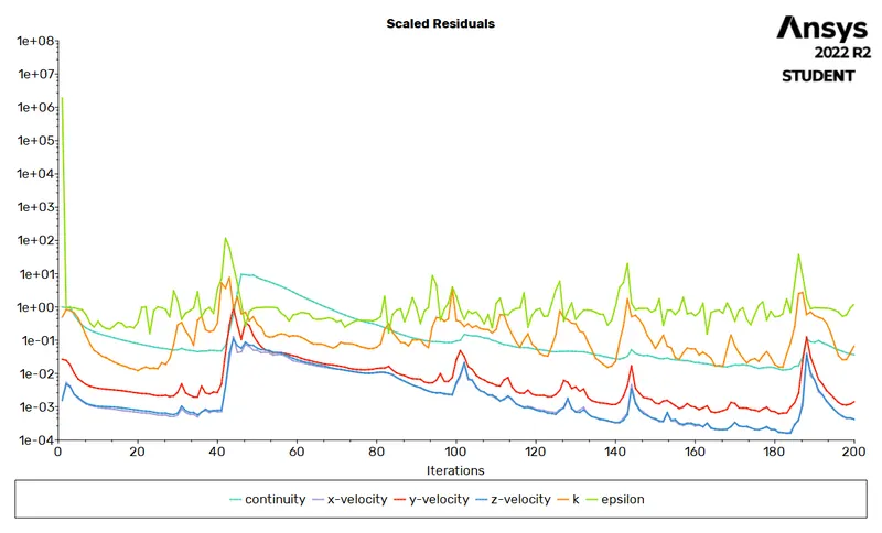
By running the simulation for 200 iterations, we obtain the following outputs.
Residuals Plot :
Mass Flow Rate :
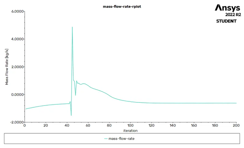
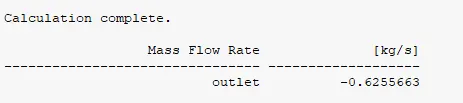
The negative sign of the mass flow rate value signifies that the mass is exiting the system.
Velocity Contour :
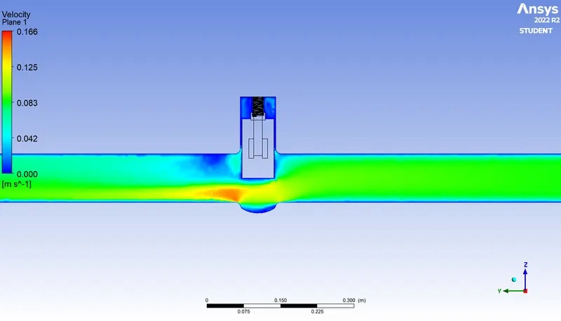
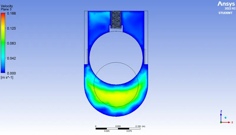
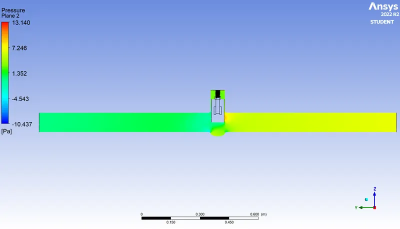
Pressure Contour :
Velocity Streamline Contour :
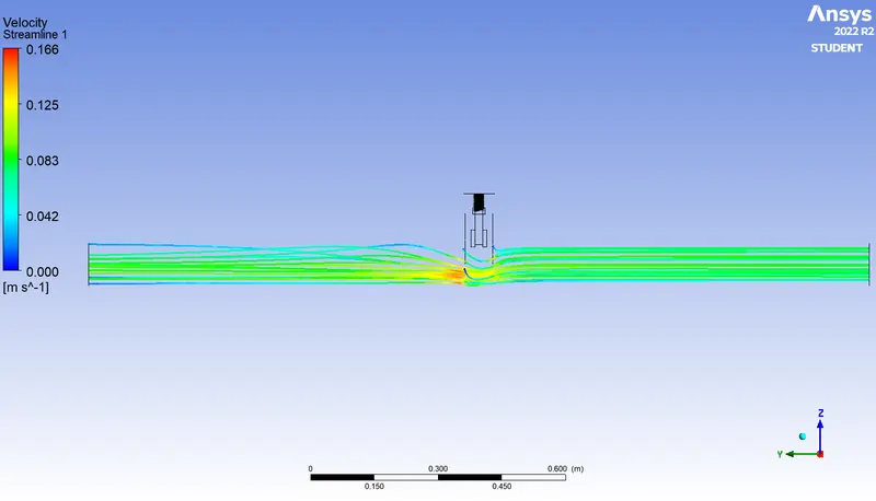
Flow Co-Efficient and Flow Factor :
In this particular case study,
`Q` = `-9.9144` `gallons`/`min`
`SG` = `1`
`DeltaP` = `0.00145` `"psi"`
Therefore,
`C_"v" = 9.9144 xx sqrt (1 / 0.00145)`
Flow Co-efficient `C_"v"` = 260.3648
Similarly,
`K_"v" = 0.865 * C_"v"`
`K_"v" = 0.865 xx 260.3648`
`therefore` Flow Factor `K_"v"` = 225.2156
Case – 7 : 70 mm Disc Lift
In this case study, we raise the gate disc up by 70 mm with respect to its initial position and we study the effects of this change on the mass flow rate.
The cross section of the lifted gate disc is represented as,
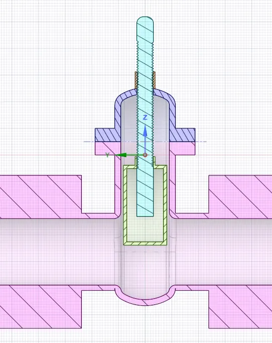
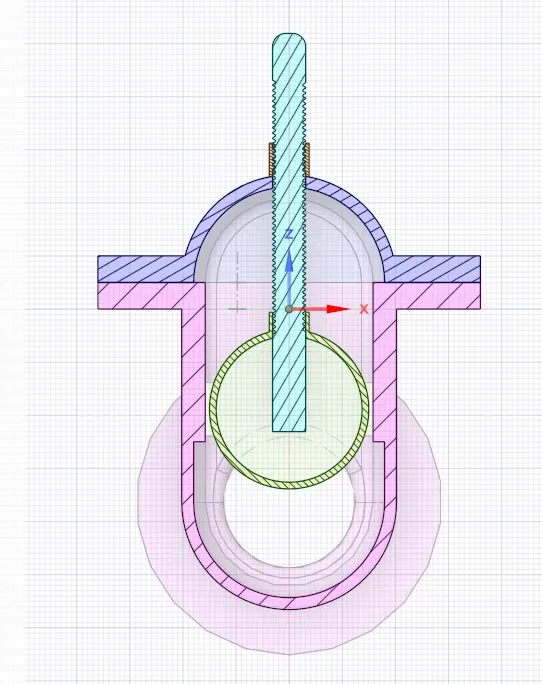
By running the simulation for 200 iterations, we obtain the following outputs.
Residuals Plot :
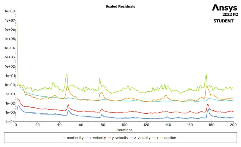
Mass Flow Rate :
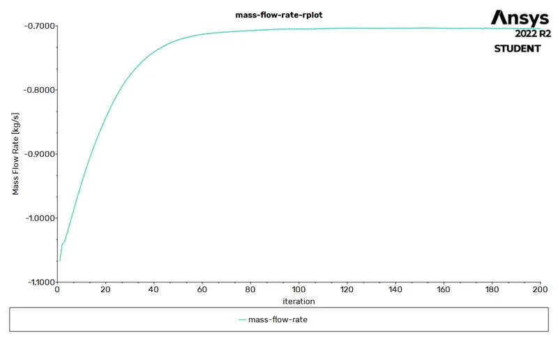
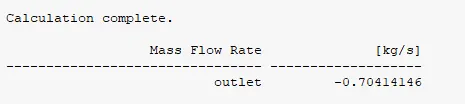
The negative sign of the mass flow rate value signifies that the mass is exiting the system.
Velocity Contour :
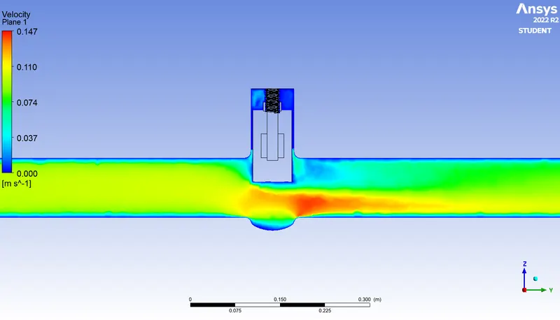
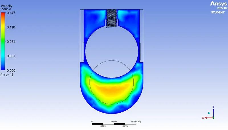
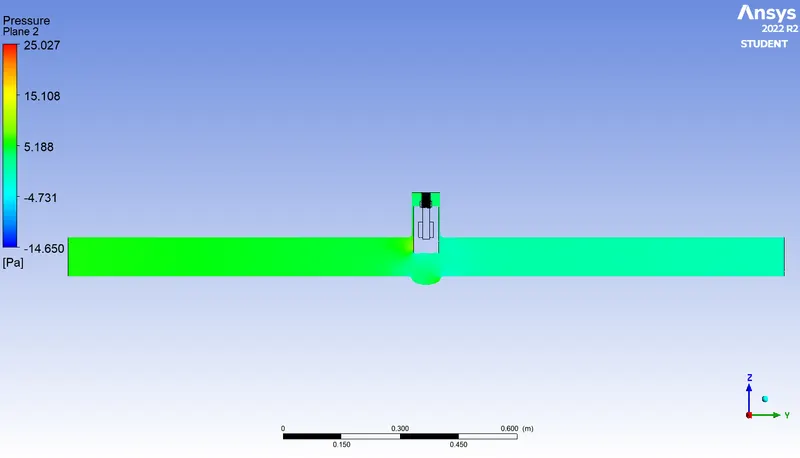
Pressure Contour :
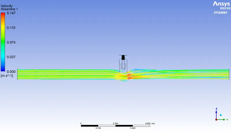
Velocity Streamline Contour :
Flow Co-Efficient and Flow Factor :
In this particular case study,
`Q` = `-11.1602` `gallons`/`min`
`SG` = `1`
`DeltaP` = `0.00145` `"psi"`
Therefore,
`C_"v" = 11.1602 xx sqrt (1 / 0.00145)`
Flow Co-efficient `C_"v"` = 293.0812
Similarly,
`K_"v" = 0.865 * C_"v"`
`K_"v" = 0.865 xx 293.0812`
`therefore` Flow Factor `K_"v"` = 253.5152
Case – 8 : 80 mm Disc Lift
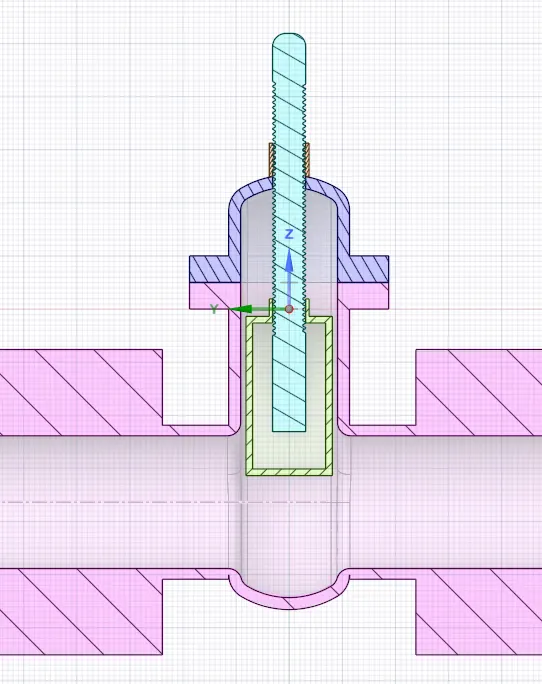
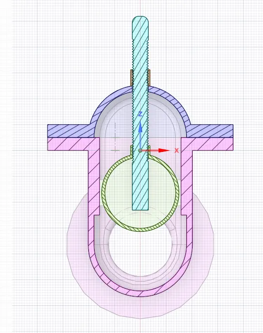
In this final case study, we raise the gate disc up by 80 mm with respect to its initial position and we study the effects of this change on the mass flow rate.
The cross section of the lifted gate disc is represented as,
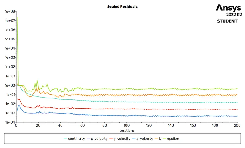
By running the simulation for 200 iterations, we obtain the following outputs.
Residuals Plot :
Mass Flow Rate :
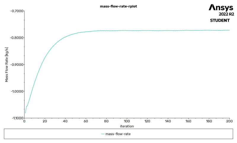
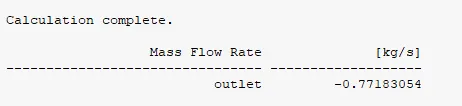
The negative sign of the mass flow rate value signifies that the mass is exiting the system.
Velocity Contour :
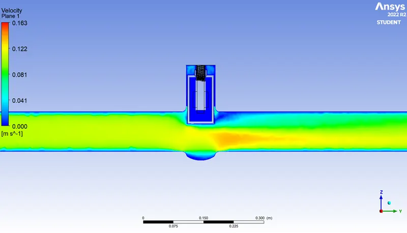
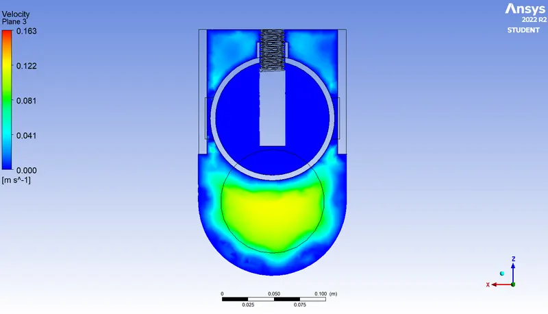
Velocity Streamline Contour :
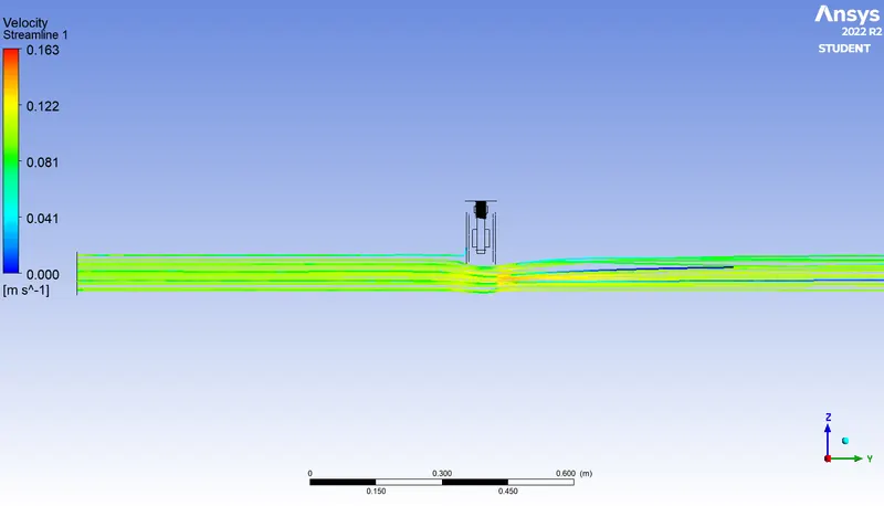
Flow Co-Efficient and Flow Factor :
In this particular case study,
`Q` = `-12.2333` `gallons`/`min`
`SG` = `1`
`DeltaP` = `0.00145` `"psi"`
Therefore,
`C_"v" = 12.2333 xx sqrt (1 / 0.00145)`
Flow Co-efficient `C_"v"` = 321.2621
Similarly,
`K_"v" = 0.865 * C_"v"`
`K_"v" = 0.865 xx 321.2621`
`therefore` Flow Factor `K_"v"` = 277.8918
PARAMETRIC STUDY TABULATION :
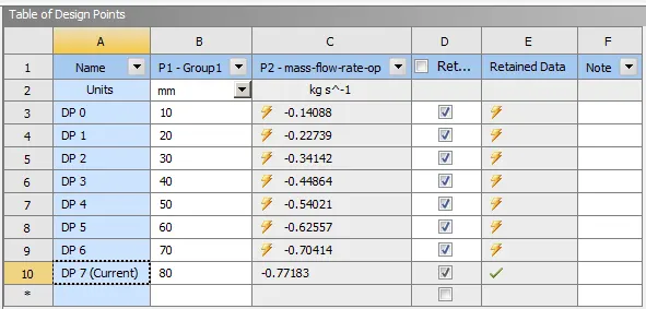
The final values of the mass flow rates of each level of lift of the gate disc have been tabulated in the parameters tab of ANSYS Workbench. Each level of lift is designated to a certain design point and updated as shown.
FINAL RESULTS :
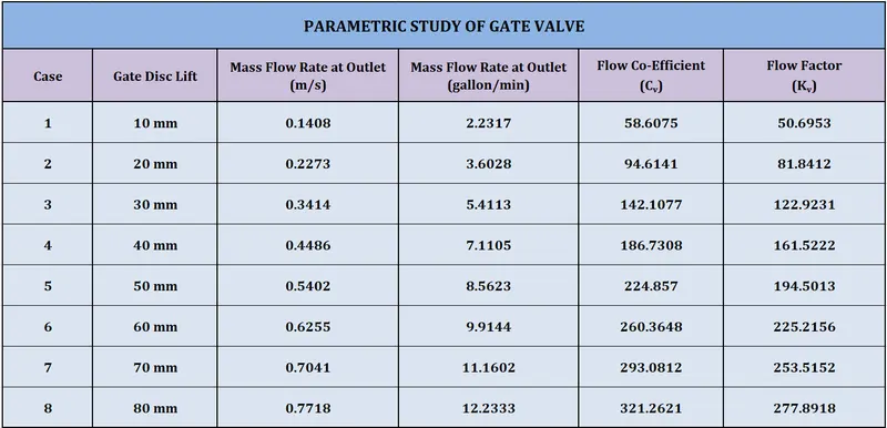
Thereby, we have successfully run the simulation for all the 8 cases – representing the different levels of gate disc lift and we obtain the final results of the simulation values as follows.
Graphical Representation :
We represent the above data in the form of line graphs and plots as follows.
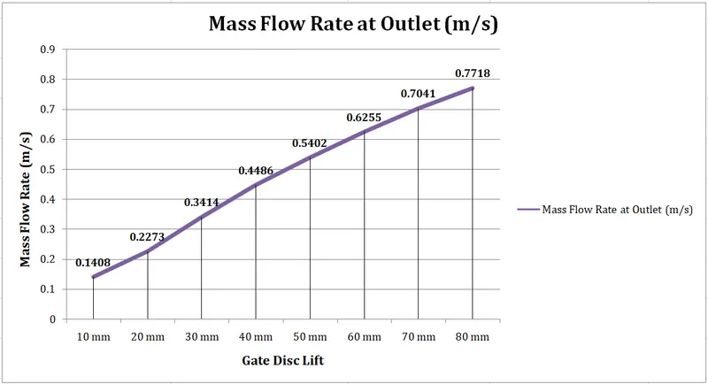
1. Gate Disc Lift vs Mass Flow Rate
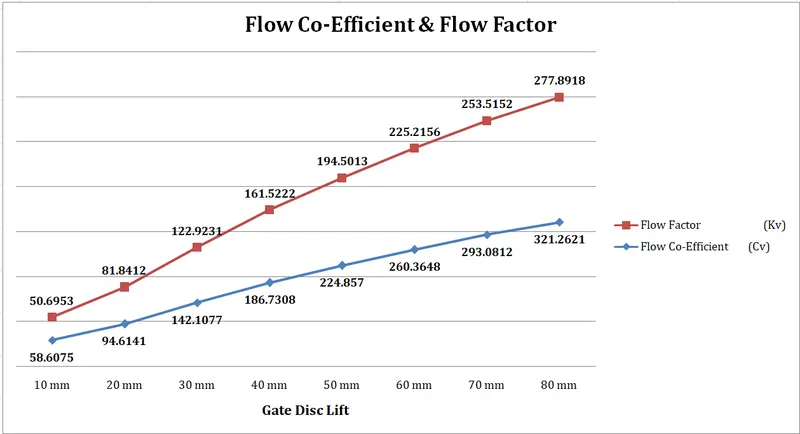
2. Variation of Flow Co-Efficient and Flow Factor with Gate Disc Lift
CONCLUSIONS :
The simulations for all 8 case studies representing the different levels of lift of the gate disc has successfully been carried out and the parametric results, along with the plots and contours have been obtained, which signify the effects of lift on the mass flow rate of the fluid at the outlet.
From the graphs and plots obtained, we can observe that with the increase in lift of the gate disc, the mass flow rate of the fluid across the outlet also increases. Therefore, the gate disc lift is directly proportional to mass flow rate. Hence, larger the gate disc opening, higher the value of mass flow rate.
Also, from the pressure plots, we can observe that as the flow progresses, there is a sudden pressure drop and the pressure reduces as it crosses the gate disc.
The level of disc lift has a direct effect on the flow co-efficient and flow factor of the gate valve. With reference to the previous calculations, as the disc lift increases, the mass flow rate increases as well. This increase in mass flow rate leads to a gradual increase in the values of flow co-efficient and flow factor, which are graphically represented above.