Damped Oscillation of a Pendulum using Python

AIM :

Write a Python program to solve the second order ODE representing the equation of motion of a simple pendulum with damping.

OBJECTIVES :

1. Write a program to solve the ODE to simulate the motion of a simple pendulum with damping.
   
   
2. Simulate the motion between 0-20 sec, for angular displacement=0, angular velocity=3 rad/sec at time t=0.
   
   
3. Create an animation video of the pendulum motion.

INTRODUCTION :

A simple pendulum is a body suspended from a fixed point so it can swing back and forth under the influence of gravity. Pendulums, like masses on a spring, are examples of simple harmonic oscillators.

It consists of a small bob of mass ‘m’ suspended at the end of a thread of length ‘l’ that is so light as to be considered massless. The period of such a device can be made longer by increasing its length, as measured from the point of suspension to the middle of the bob. A change in the mass of the bob, however, does not affect the period, provided the length is not thereby affected.

Assumptions:

• There is negligible friction from the air and the system
• The arm of the pendulum does not bend or compress and is massless
• The pendulum swings in a perfect plane
• Gravity remains constant.

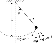
A pendulum's bob swinging is kept in motion by this force acting upon it as it moves back and forth. In pendulum motion, three forces work directly on the pendulum​: the mass of the bob, gravity and the tension in the string. Mass and gravity both work vertically downward. Since the pendulum doesn’t move up or down, the vertical component of the string tension cancels out the mass and gravity.

GOVERNING EQUATIONS :

The Ordinary Differential Equation (ODE) that represents the motion of a simple pendulum is given by,

`(d^2theta)/(dt^2) + b/m (d theta)/dt + g/L sin theta = 0`

Where,

`b` = Damping coefficient

`m` = Mass of the pendulum bob

`g` = Acceleration due to gravity

`L` = Length of massless string or rod

`theta` = Angle of pendulum

We break down the above 2^nd order ODE's into a set of 1^st order ODE's.

Considering, `theta = theta_1`

`=>` `(d theta)/dt = (d theta_1)/dt = theta_2` - equation (1)

Also, `(d^2 theta)/dt^2 = (d^2 theta_1)/dt^2` {`because theta = theta_1`}

`=>` `(d^2 theta)/dt^2 = d/dt((d theta_1)/dt) = d/dt (theta_2)`

If `theta = theta_1`, the simple pendulum equation becomes,

`(d^2theta_1)/(dt^2) + b/m (d theta_1)/dt + g/L sin theta_1 = 0`

This means that, to solve the original 2^nd order ODE, we have created two 1^st order ODE's which are,

`(d theta_1)/dt = theta_2` and `(d theta_2)/(dt) = - b/m (theta_2) - g/L sin theta_1`

Therefore, in matrix form, the solution vector is given by,

`d/(dt) [(theta_1), (theta_2)] = [(theta_2),(-b/m theta_2 - g/L sintheta_1)]`

PROGRAM & EXPLANATION :

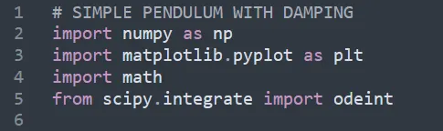
In the first step of the program, we import the necessary modules into Python as shown. Here, we import the “odeint” library, which is a collection of advanced numerical algorithms to solve initial-value problems of ordinary differential equations.

Function Definition :

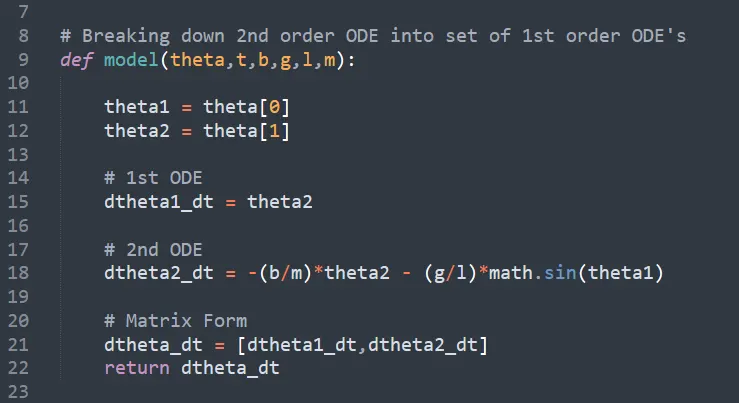
In this step, we break down the 2^nd order ODE into a set of 1^st order ODE equations for simplification.

• We define a function which takes the input values of `theta`, `t` , `b`, `g` , `l`, `m` and returns the `(d theta)/dt` array.
  
  
• This array contains two 1^st order ODE equations, which the 2^nd order ODE has been broken down into, as shown in the above derivation.

Defining Input & Initial Conditions :

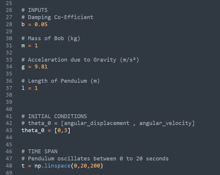
• Here, we define the input values of the various parameters of the pendulum such as the Damping Co-Efficient (b), Mass of Bob (m), Acceleration due to Gravity (g) and the Length of the Pendulum (l).
  
  
  
• Further, we define the initial condition values of the angular displacement as 0 and angular velocity as 3 rad/sec.
  
  
  
• As we animate the pendulum motion from 0 to 20 seconds, we define that as the time span.

Solving ODE Equation & Plotting Results :

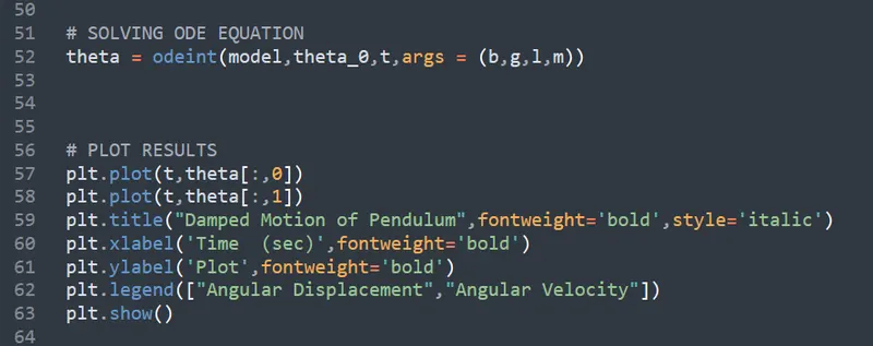
• Finally, we solve the ODE equations by using the “odeint” inbuilt function and providing the input values of initial conditions and the defined pendulum parameters.
  
  
  
• The above obtained values are plotted as a function of time and thereby obtaining our plot of change in frequency of oscillations of the pendulum with respect to time.

Pendulum Animation :

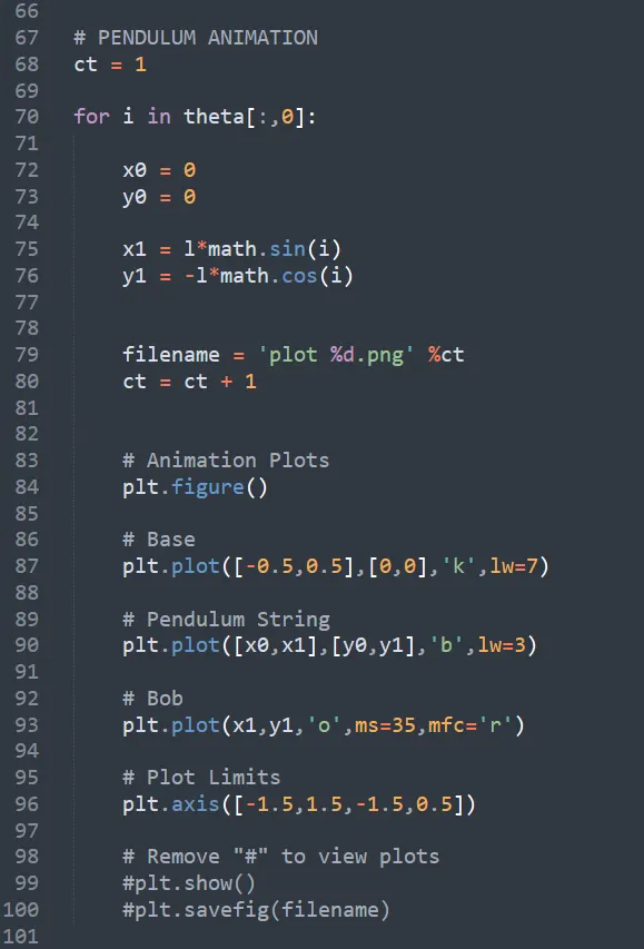
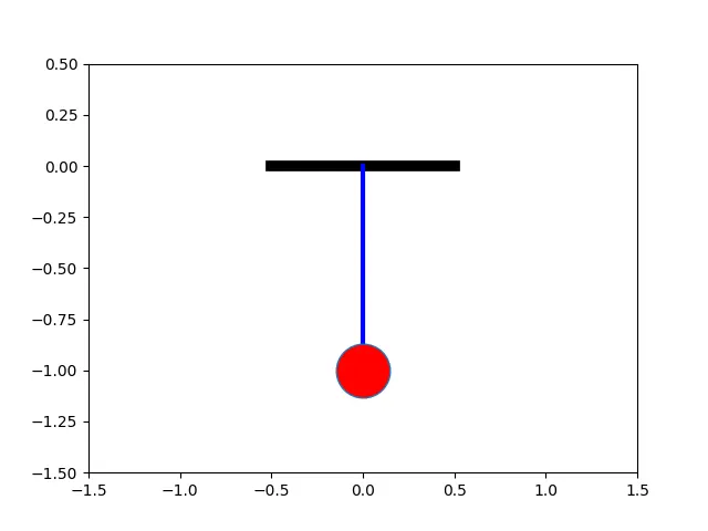
Finally, we write a code to obtain an animation of the damped motion of the pendulum.

• Firstly, we plot the fixed base to which the pendulum is attached.
  
  
  
• Next, we plot the string of length ‘l’, which oscillates at angles of `sintheta` and `costheta`, with respect to the centre. One end of the string is fixed to the base where as the other end is free to move.
  
  
  
• The free end of the string is attached to a bob of mass ‘m’. With respect to the oscillation of the string, the bob is plotted as well and thereby obtaining our final animation plots of the motion of the pendulum.

RESULTS :

By running the above program code, we obtain the following outputs.

1. Oscillations Plot

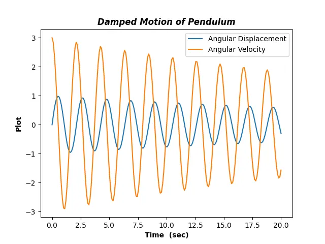
The below plot represents the variation of angular displacement and angular velocity with respect to time.

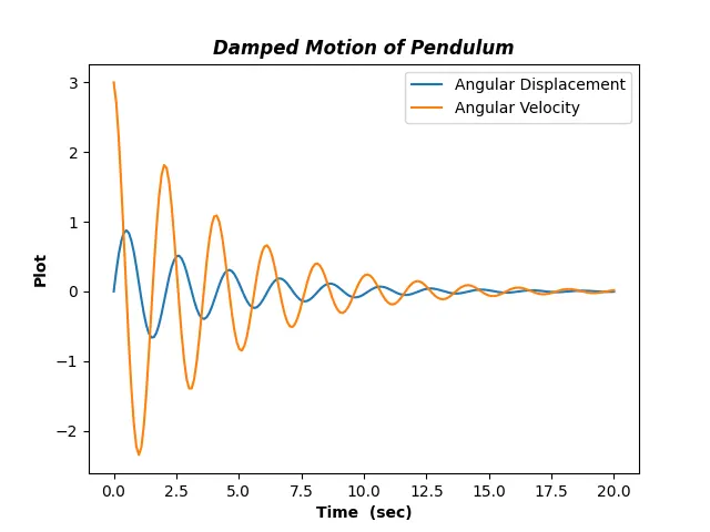
By increasing the value of damping co-efficient (b = 0.5), the damping effect on the pendulum is increased and we thereby obtain the plot as follows.

2. Pendulum Animation

The final animation of the damped motion of a pendulum is obtained as follows.

Final Program :

# SIMPLE PENDULUM WITH DAMPING
import numpy as np
import matplotlib.pyplot as plt
import math
from scipy.integrate import odeint


# Breaking down 2nd order ODE into set of 1st order ODE's
def model(theta,t,b,g,l,m):

    theta1 = theta[0]
    theta2 = theta[1]

    # 1st ODE
    dtheta1_dt = theta2

    # 2nd ODE
    dtheta2_dt = -(b/m)*theta2 - (g/l)*math.sin(theta1)

    # Matrix Form
    dtheta_dt = [dtheta1_dt,dtheta2_dt]
    return dtheta_dt



# INPUTS
# Damping Co-Efficient
b = 0.05

# Mass of Bob (kg)
m = 1

# Acceleration due to Gravity (m/s²)
g = 9.81

# Length of Pendulum (m)
l = 1



# INITIAL CONDITIONS
# theta_0 = [angular_displacement , angular_velocity]
theta_0 = [0,3]


# TIME SPAN
# Pendulum oscillates between 0 to 20 seconds
t = np.linspace(0,20,200)


# SOLVING ODE EQUATION
theta = odeint(model,theta_0,t,args = (b,g,l,m))



# PLOT RESULTS
plt.plot(t,theta[:,0])
plt.plot(t,theta[:,1])
plt.title("Damped Motion of Pendulum",fontweight='bold',style='italic')
plt.xlabel('Time  (sec)',fontweight='bold')
plt.ylabel('Plot',fontweight='bold')
plt.legend(["Angular Displacement","Angular Velocity"])
plt.show()



# PENDULUM ANIMATION
ct = 1

for i in theta[:,0]:

    x0 = 0
    y0 = 0

    x1 = l*math.sin(i)
    y1 = -l*math.cos(i)


    filename = 'plot %d.png' %ct
    ct = ct + 1


    # Animation Plots
    plt.figure()

    # Base
    plt.plot([-0.5,0.5],[0,0],'k',lw=7)

    # Pendulum String
    plt.plot([x0,x1],[y0,y1],'b',lw=3)

    # Bob
    plt.plot(x1,y1,'o',ms=35,mfc='r')

    # Plot Limits
    plt.axis([-1.5,1.5,-1.5,0.5])

    # Remove "#" to view plots
    #plt.show()
    #plt.savefig(filename)
 

CONCLUSIONS :

The Python code representing the damped motion of a pendulum has been written and the outputs of frequency of oscillations and the pendulum animation have successfully been obtained.

From the frequency plot, we can observe that as the pendulum oscillates for a longer time, the frequency of oscillation gradually decreases till the pendulum comes to a complete stop. This type of motion of the pendulum is referred to as Simple Harmonic Motion (SHM).

From the plots, it can also be concluded that by increasing the value of the damping co-efficient, the oscillation frequency sharply reduces with respect to time due to higher damping effects acting on the pendulum. Therefore, higher the damping co-efficient, sooner the pendulum comes to a rest.