Week 1- Mixing Tee
AIM :
To set up steady-state simulations to compare the mixing effectiveness of a short and long tee - junctions.
OBJECTIVES :
- The main objective of this challenge is to set up steady-state simulations to compare the mixing effectiveness of long and short tee – junctions, when the hot inlet temperature is 360C & the cold inlet is at 190C.
- To carry out the simulation for two cases,
Case – 1 :
• Short mixing tee with a hot inlet velocity of 3 m/s.
• Momentum ratio of 2, 4.
Case – 2 :
• Long mixing tee with a hot inlet velocity of 3 m/s.
• Momentum ratio of 2, 4.
- Use the realizable k-ε and k–ω SST model for the first case and based on your judgment use the more suitable model for further cases. Giving the reason for choosing a suitable model.
- In a table, compare the following values from the 2 cases.
i.) Cell count
ii.) Average outlet temperature
iii.) Number of iterations for convergence
INTRODUCTION :
Tee junctions are flow control devices, which are used for the efficient mixing of two fluids. It is called a tee junction because the angle between the fluids getting mixed is `90^o`.
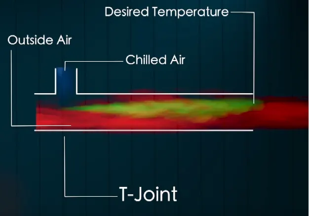
Mixing Tees utilizes a specifically engineered internal geometry to efficiently mix two fluid streams into one combined stream. Mixing tees are widely used in the petrochemical, HVAC industry etc., in which two fluid streams with different physical and/or chemical properties mix together.
k-ε turbulence model (Realizable) :
k-epsilon (k-ε) turbulence model is the most common model used in computational fluid dynamics (CFD) to simulate mean flow characteristics for turbulent flow conditions. It is a two-equation model. That means that in addition to the conservation equations, it solves two transport equations (PDE's), which account for the history effects like convection and diffusion of turbulent energy. The two transported variables are turbulent kinetic energy (k), which determines the energy in turbulence, and turbulent dissipation rate (ε), which determines the rate of dissipation of turbulent kinetic energy. It belongs to the Reynolds-Averaged Navier Stokes (RANS) family of turbulence models.
Unlike other turbulence models, k-ε model focuses on the mechanisms that affect the turbulent kinetic energy. The underlying assumption of this model is that the turbulent viscosity is isotropic, in other words, the ratio between Reynolds stress and mean rate of deformations is the same in all directions.
An immediate benefit of the realizable k-ɛ model is that it exhibits superior performance for flows involving rotation, boundary layers under strong adverse pressure gradients, separation, and recirculation. In virtually every measure of comparison, Realizable k-ɛ demonstrates a superior ability to capture the mean flow of the complex structures.
k–ω turbulence model (SST) :
In computational fluid dynamics, the k–omega (k–ω) turbulence model is a common two-equation turbulence model, that is used as an approximation for the Reynolds-Averaged Navier–Stokes equations (RANS equations). The model attempts to predict turbulence by two partial differential equations for two variables, k and ω, with the first variable being the turbulence kinetic energy (k) while the second (ω) is the specific rate of dissipation (of the turbulence kinetic energy k into internal thermal energy).
The SST k-ω turbulence model is a two-equation eddy-viscosity model which has become very popular. The shear stress transport (SST) formulation combines the best of two worlds. The use of a k-ω formulation in the inner parts of the boundary layer makes the model directly usable all the way down to the wall through the viscous sub-layer. Hence the SST k-ω model can be used as a Low-Re turbulence model without any extra damping functions. The SST formulation also switches to a k-ε behaviour in the free-stream and thereby avoids the common k-ω problem that the model is too sensitive to the inlet free-stream turbulence properties. The SST k-ω model often merited for its good behaviour in adverse pressure gradients and separating flow.
The SST k-ω model does produce a bit too large turbulence levels in regions with large normal strain, like stagnation regions and regions with strong acceleration. This tendency is much less pronounced than with a normal k-ε model though.
SPECIFICATIONS & GIVEN DATA :
In this challenge, we have to simulate the steady state mixing in a short and long tee joint.
- Hot Inlet Temperature = `36^o C`
- Cold Inlet Temperature = `19^o C`
Turbulence Models to be used and results to be compared,
- Realizable k-ε turbulence model
- k–ω SST turbulence model
Simulation cases,
Case – 1 :
- Short mixing tee with a hot inlet velocity of 3m/s.
- Momentum ratio of 2, 4.
Case – 2 :
- Long mixing tee with a hot inlet velocity of 3m/s.
- Momentum ratio of 2, 4.
Where,
`"Momentum Ratio" = "Velocity at Cold Inlet" / "Velocity at Hot Inlet"`
Comparisons to be done from values of 2 cases,
- Cell count
- Average outlet temperature
- Number of iterations for convergence
Expected results:
- Velocity and temperature contour plots on the cut planes along and across the pipe.
- Velocity and temperature line plots along and across the length of the pipe.
- Mesh Independence study for any one case.
- The effect of length and momentum ratio on results.
- Convergence plots for each simulation.
CASE SETUP :
For this simulation, we are going to be setting up two cases,
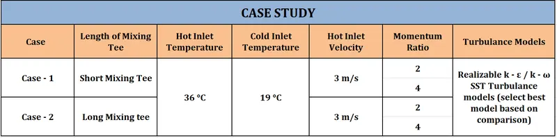
SIMULATION PROCEDURE :
For this challenge, we are going to use the ANSYS Student Version software to simulate the flow through the tee joint. The workflow procedure of the simulation is as shown below.

The simulation is carried out in the ANSYS Workbench software in 5 steps namely,
- Geometry
- Meshing
- Setup
- Solution
- Results
General Simulation Setup :
We are going to begin the simulation by opening the ANSYS Workbench software. From the toolbox at the left hand side, we select the Fluid Flow (Fluent) module to head further with the simulation.

The next step is creating the geometry.
CASE – 1 : SHORT MIXING TEE
We are going to carry out this case study of a short mixing tee to compare the results obtained from the k-ε and k–ω turbulence models, to decide which is more optimal.
1. GEOMETRY
In this step, we are going to import the geometry on which we are going to carry out the simulation.
Software Used : ANSYS SpaceClaim
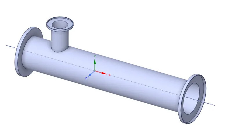
In the first step, we are going to import the step - file/solid model into SpaceClaim. The tee geometry is as shown below.
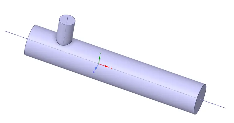
Next, we prepare the geometry by performing volume extraction to extract the wet volume of the model. Wet volume refers to the surface where the fluid interacts with the model. This extraction is done to remove all the additional surfaces, except the wet volume surface, as that is the only surface under study. The volume extracted geometry is as shown below.
We use the “suppress for physics” function to make sure the solid part is not loaded for meshing.
2. MESHING
The next step in the simulation is creating a meshed model of the geometry obtained.
Software Used : ANSYS Meshing (CFD PrepPost)
Before meshing, we first create the named selection faces to name the faces and walls of the geometry, being the x – inlet, y – inlet, outlet and the walls of the geometry.

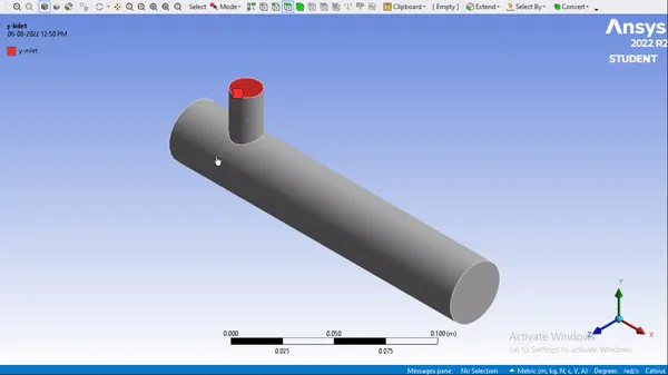
After creating the named selection faces, we then move on to generate the meshing for the geometry. The software automatically generates the mesh by the principle of bounding box, which fits the geometry or all of its components in the smallest size box which it can be enclosed in. From the dimensions of this box, the meshing is generated.
To get a fine mesh, we change the default element size to 0.003.
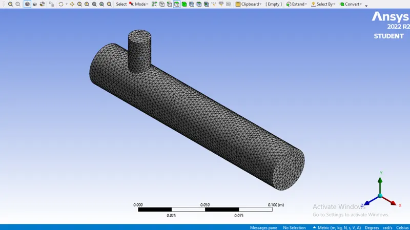
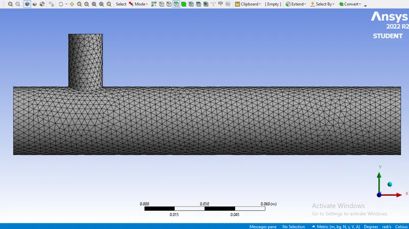
`360^o` View of Meshed Model :
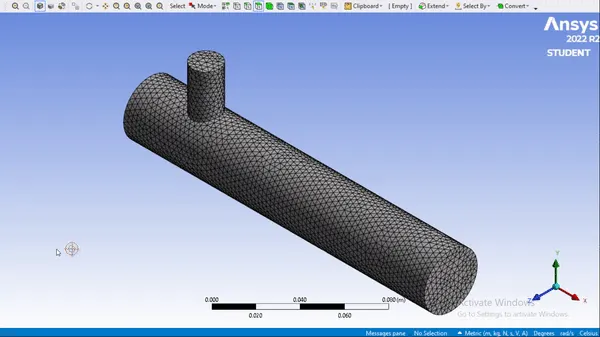
Next, we use the section plane function to create a cross section of the geometry, so as to get a better understanding of the generated meshing.
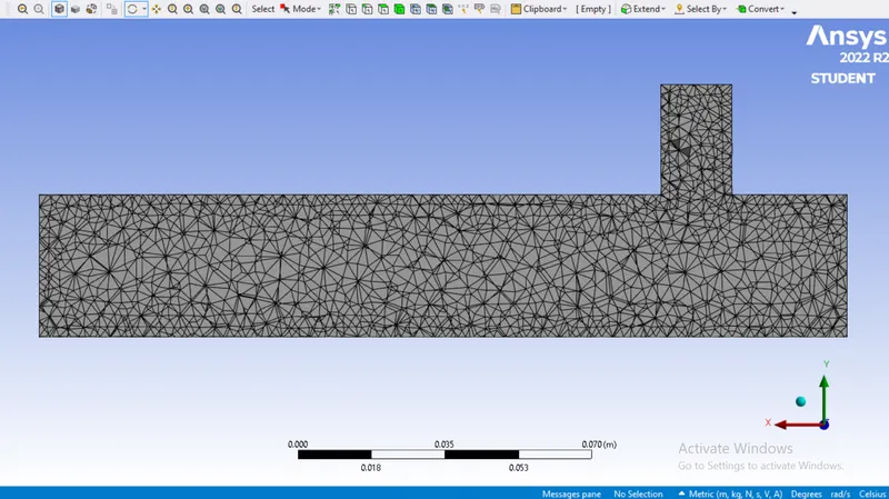
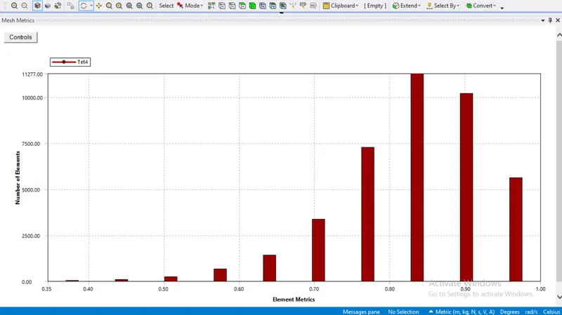
To evaluate the mesh quality, we use the mesh metric function to check the element quality of the meshing. We have to make sure that the quality of the mesh is not under 5%.
3. SETUP
In this step, we are going to define the turbulence models used to run the simulation calculations for this respective case.
Software Used : ANSYS Fluent
Here, we are going to conduct a study to compare the performance of 2 RANS based turbulence models - realizable k-ɛ model and SST k-ω turbulence model, respectively.
- As we are solving for temperature, we use the energy equation as well.
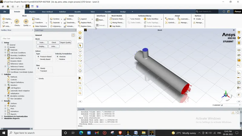
- Before defining the turbulence models, we perform a mesh check test to determine the quality of the mesh.
- We select a pressure - based steady time solver with absolute velocity formulation, to set up the turbulence models.
Case 1.1 :
Length : Short Tee Joint
Hot Inlet Temperature : 360C
Cold Inlet Temperature : 190C
Turbulence Model : Realizable k-ɛ / SST k-ω Turbulence Models (Comparison Study)
Hot Inlet Velocity : 3 m/s
Momentum Ratio : 2
Cold Inlet Velocity : 6 m/s
For this case, we are going to conduct a case study to compare the results of the realizable k-ɛ model to the k-ω turbulence model so as to determine which is the best model for this simulation. The results of the study are as shown below.
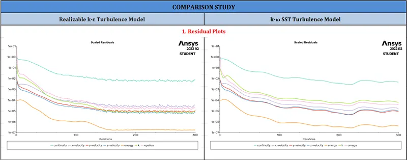
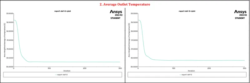
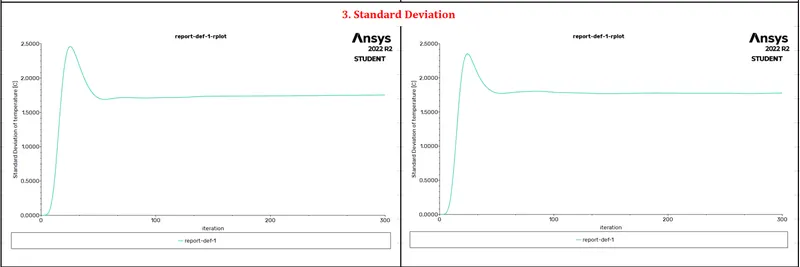
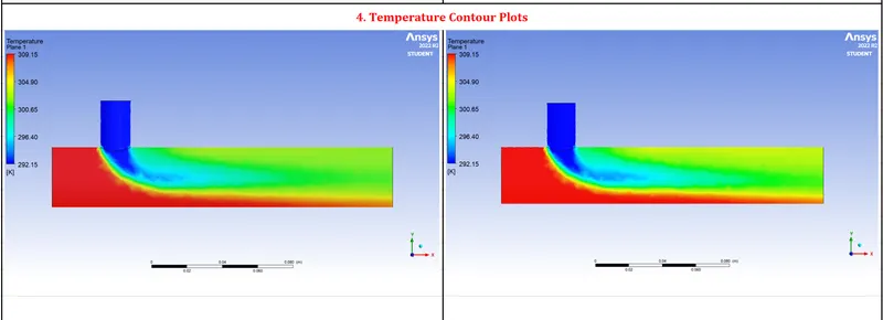
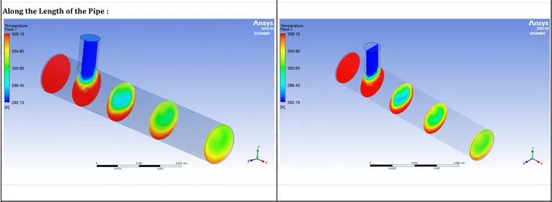
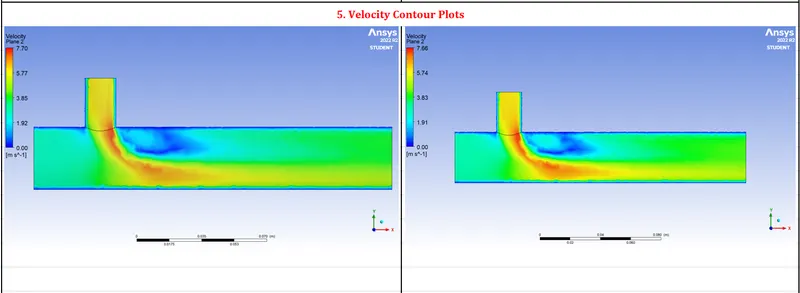
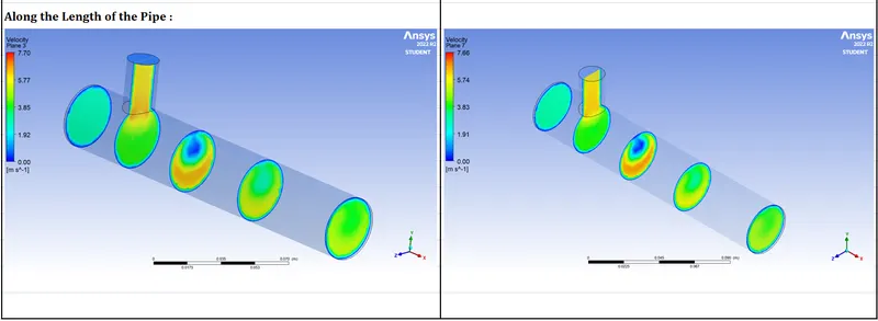

From the above comparison chart, we can observe that the k-ɛ model has lesser standard deviation when compared to the k-ω model. This means that, better mixing is achieved with a lesser standard deviation value. Therefore, we will use the realizable k-ɛ turbulence model for the further cases.
Case 1.2 :
Length : Short Tee Joint
Hot Inlet Temperature : 360C
Cold Inlet Temperature : 190C
Turbulence Model : Realizable k-ɛ Turbulence Model
Hot Inlet Velocity : 3 m/s
Momentum Ratio : 4
Cold Inlet Velocity : 12 m/s
For this case study, we are going to increase the cold inlet velocity and we are going to study how the average outlet temperature changes as a function of the cold inlet velocity.
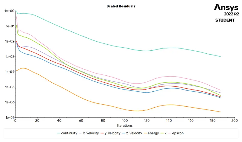
Residual Plot :
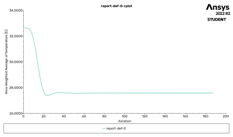
Area Weighted Average Temperature Plot :
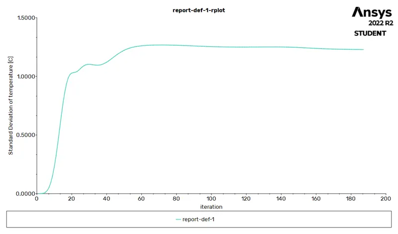
Standard Deviation :
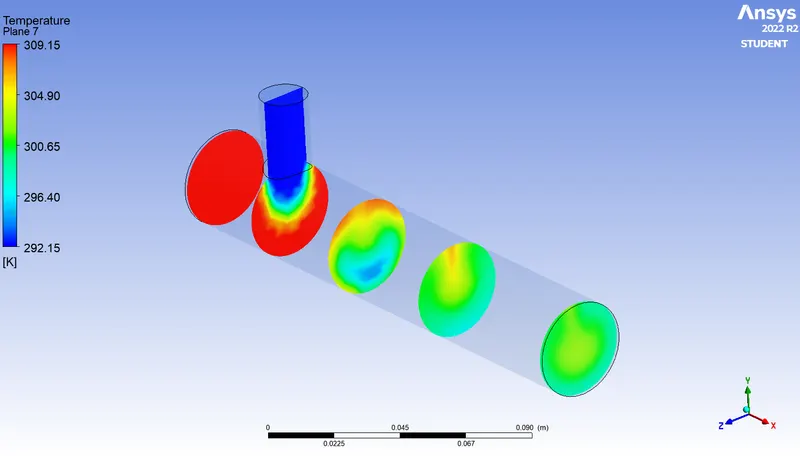
Temperature Contour Plot :
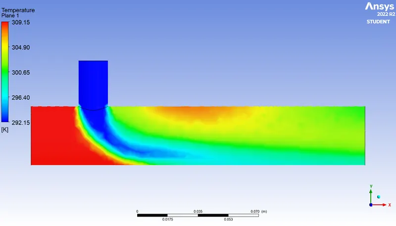
Along the length of the pipe :
Velocity Contour Plot :
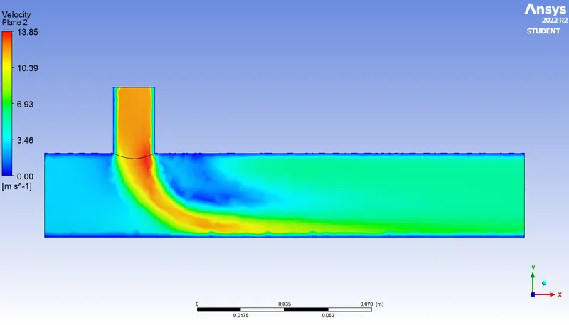
Along length of the pipe :
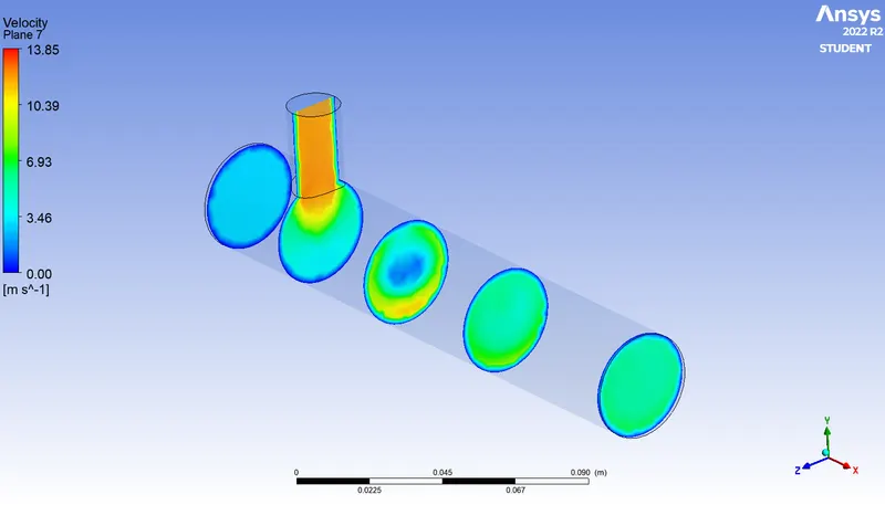
Output Parameters :
Average Temperature at Outlet = 27.6029 0C
Standard Deviation = 1.2263 0C
Number of iterations to converge = 187.
From the above results, we can observe that, with the increase in cold inlet velocity, the average temperature at the outlet also substantially decreases. Thereby, for a short tee joint, we can conclude that the increase in cold inlet velocity leads to more efficient cooling.
CASE – 2 : LONG MIXING TEE
In this case study, we are going to run the simulation for a long mixing tee to observe whether the change in length of the tee joint affects the outputs of the simulation.
1. GEOMETRY
The geometry or model of the long mixing tee is as shown below.
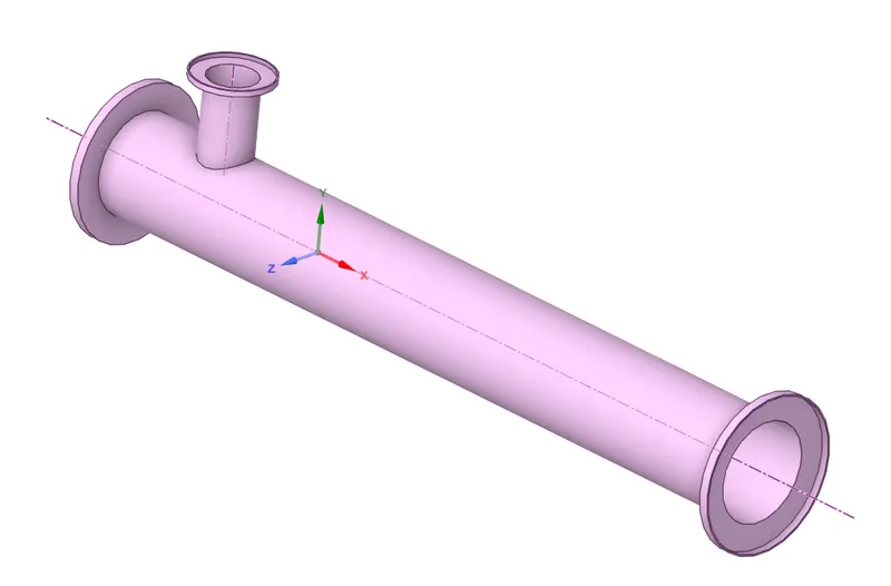
We perform volume extraction for the above geometry to extract the wet volume, which we will further use to run the simulation.
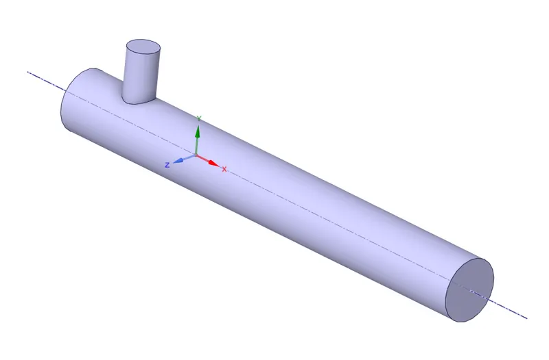
2. MESHING
Before generating the mesh, we first create the named selection faces to define the hot inlet, cold inlet, outlet and the walls of the geometry. Next, we set the default element size to 0.003 and we generate the mesh as shown below.
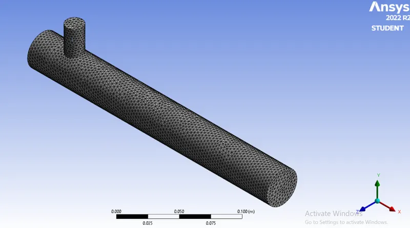
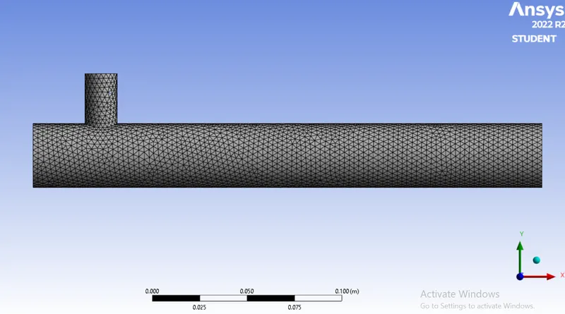
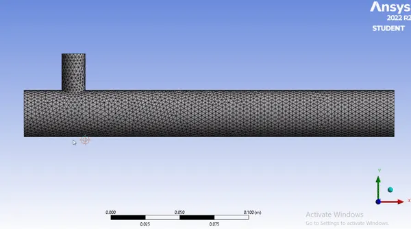
`360^o` View of Meshed Model :
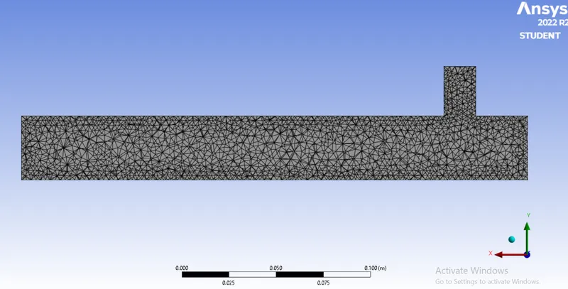
We create a section plane of the meshed geometry to study the generated mesh in detail.
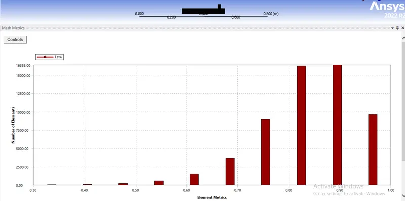
Finally, we check the element quality of the mesh using the mesh metric function, to make sure the mesh quality does not go under 5%.
Case 2.1 :
Length : Long Tee Joint
Hot Inlet Temperature : 360C
Cold Inlet Temperature : 190C
Turbulence Model : Realizable k-ɛ Turbulence Model
Hot Inlet Velocity : 3 m/s
Momentum Ratio : 2
Cold Inlet Velocity : 6 m/s
With reference to the above mentioned boundary conditions, at the inlet and the outlet, we are going to run the simulation for these values.
3. SETUP & SOLUTION
- First, we are going to define a realizable k-ɛ turbulence model with standard wall functions, with respect to which the simulation is run.
- We define the working fluid as air.
- Similarly, we are also going to setup the boundary conditions for the same, whose magnitude is normal to the boundary.
- In the solution tab, we define the reports which we need to obtain from this case study.
- Finally, we are going to initialize the simulation by hybrid initialization and run it for 300 iterations and thereby obtaining our output plots and solution.
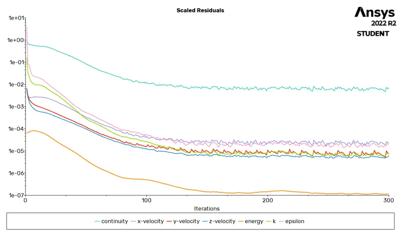
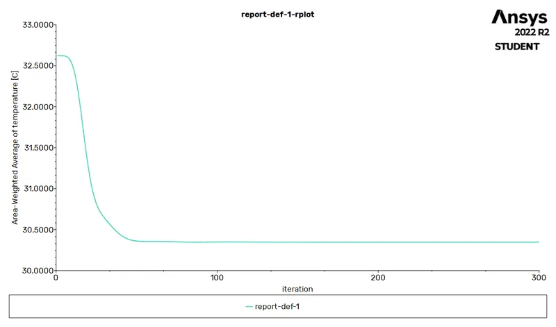
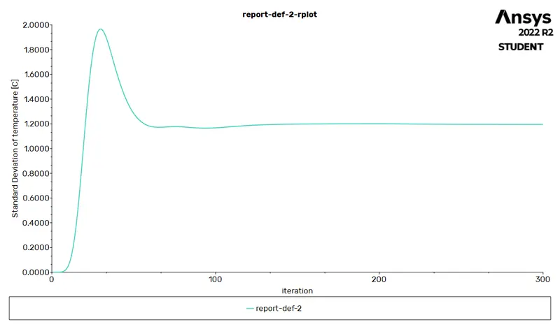
We obtain the respective plots as follows,
Residual Plot :
Area Weighted Average Temperature Plot :
Standard Deviation :
4. RESULTS
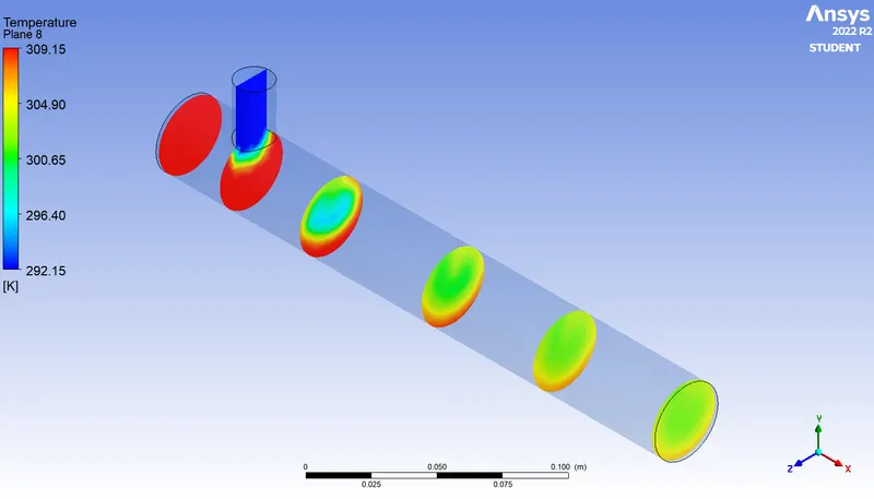
From the obtained calculations, we then post – process the solution to a visual representation form using the ANSYS CFD – Post software. The outputs are as follows.
Temperature Contour Plot :
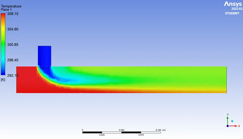
Along length of the pipe :
Velocity Contour Plot :
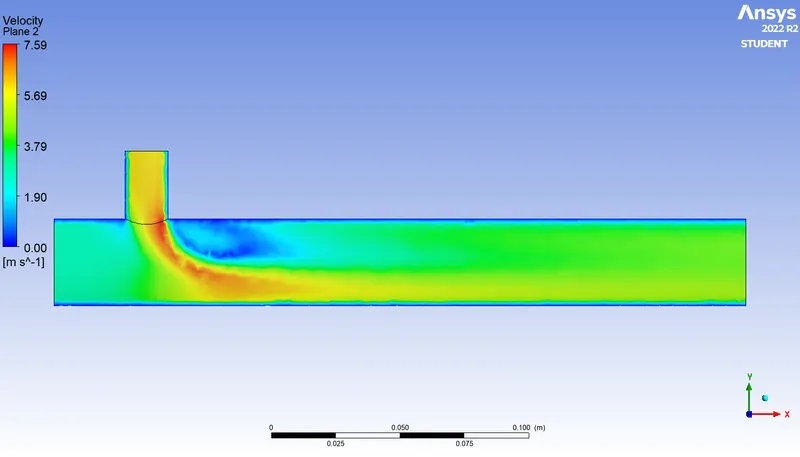
Along length of the pipe :
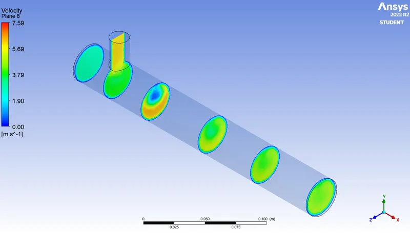
Output Parameters :
Average Temperature at Outlet = 30.3435 0C
Standard Deviation = 1.1914 0C
Number of iterations to converge = 250 ~ 350.
Case 2.2 :
Length : Long Tee Joint
Hot Inlet Temperature : 360C
Cold Inlet Temperature : 190C
Turbulence Model : Realizable k-ɛ Turbulence Model
Hot Inlet Velocity : 3 m/s
Momentum Ratio : 4
Cold Inlet Velocity : 12 m/s
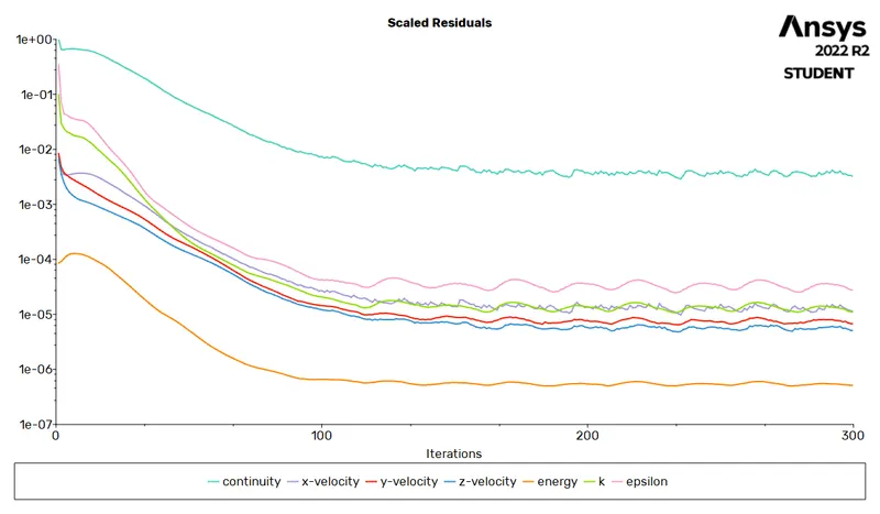
In this case, we are going to simulate the flow for a momentum ratio of 4, which increases the velocity at the cold inlet and thereby observe if there is any difference.
By running the simulation, we obtain the respective plots.
Residual Plot :
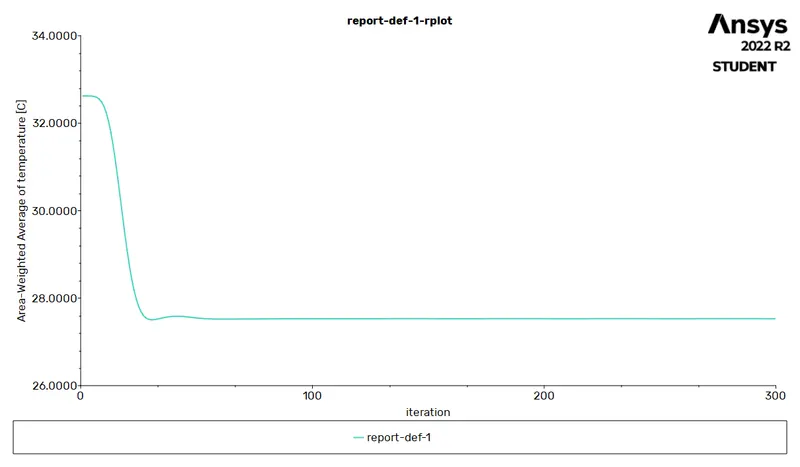
Area Weighted Average Temperature Plot :
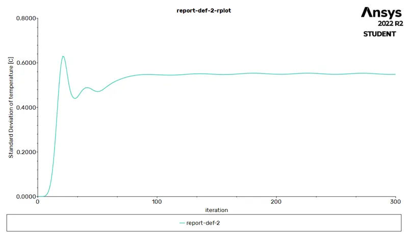
Standard Deviation :
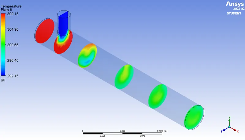
Temperature Contour Plot :
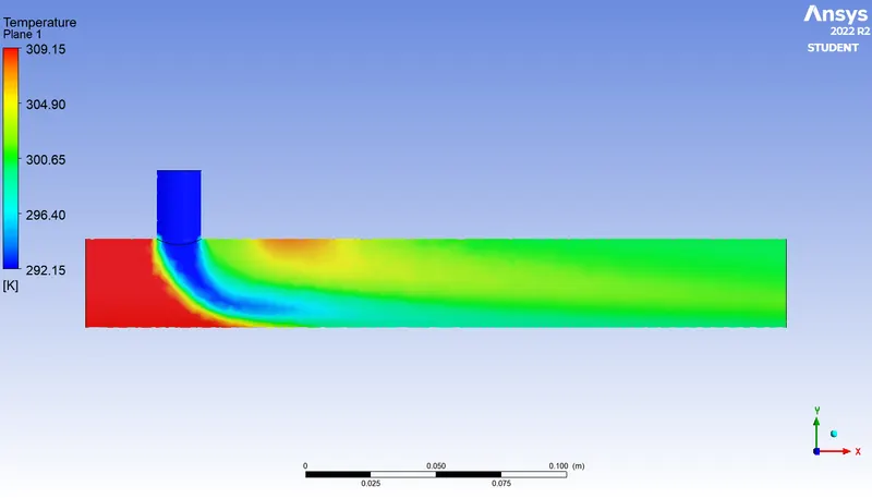
Along length of the pipe :
Velocity Contour Plot :
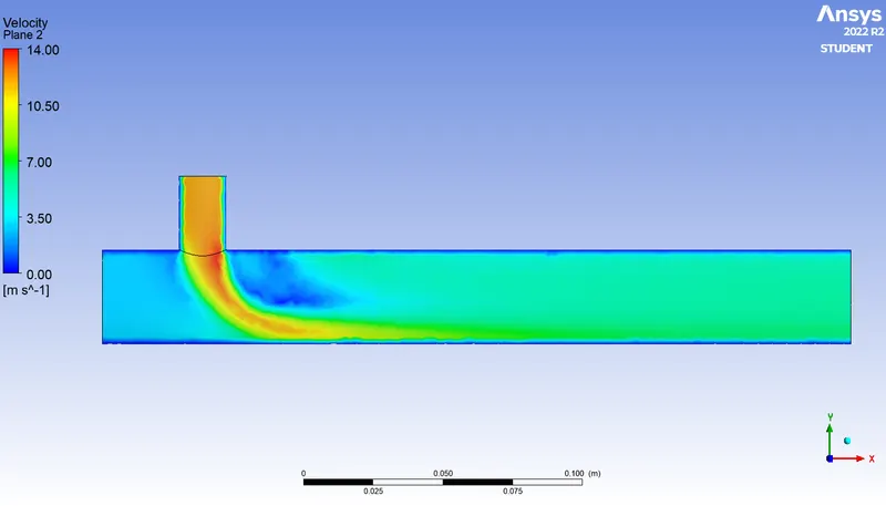
Along length of the pipe :
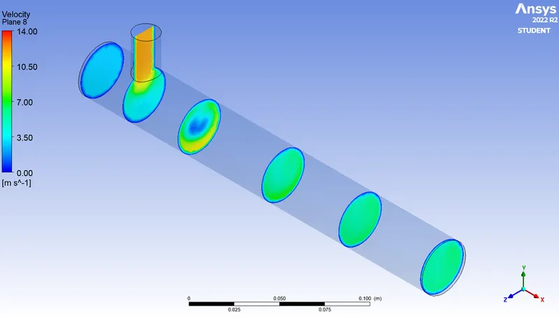
Output Parameters :
Average Temperature at Outlet = 27.5217 0C
Standard Deviation = 0.5507 0C
Number of iterations to converge = 250 ~ 350.
From the above case study, we can observe that by increasing the cold inlet velocity, we obtain more efficient cooling at the outlet. This also leads to a low value of standard deviation, which means that there is effective mixing as well.
VALIDATION :
In this step, we are going to validate our results by comparing the results obtained from the simulation with our analytical results.
Analytical Solution :
We are considering our working fluid as air, whose density (`rho`) is 1.225 kg/m.
We have the formula,
`T_"mixture" = (m_"hot" ** T_"hot" + m_"cold" ** T_"cold")/(m_"hot" + m_"cold")`
Where,
`T_"mixture" =` Average Temperature of Fluid at Outlet
`m_"hot" =` Mass Flow Rate of Hot Fluid = `rho*A*V_"hot"`
`T_"hot" =` Temperature at Hot Inlet
`m_"cold" =`Mass Flow Rate of Cold Fluid = `rho*A*V_"cold"`
`T_"cold" =` Temperature at Cold Inlet
Calculations :
Considering the 4 cases of the short and long tee joints,
Case 1.1 :
`T_"hot" = 36^o C` ; `V_"hot" = 3` m/s ; `T_"cold" = 19^o C` ; `V_"cold" = 6` m/s ;
`A_"hot" = 891.86` `mm^2` ; `A_"cold" = 221.42` `mm^2` ; `rho_"air" = 1.225` kg/m
Mass Flow Rates,
`m_"hot" = rho*A*V_"hot"`
`= 1.225 xx 891.86 xx 3`
`m_"hot" = 3277.58` kg/s
`m_"cold" = rho*A*V_"cold"`
`= 1.225 xx 221.42 xx 6`
`m_"cold" = 1627.43` kg/s
Average Outlet Temperature,
`T_"mixture" = ((3277.58 xx 36) + (1627.43 xx 19))/(3277.58 + 1627.43)`
`therefore` `T_"mixture" = 30.359 ^o C`
Similarly for the other cases, we get
Case 1.2 : `T_"mixture" = 27.529^o C`
Case 2.1 : `T_"mixture" = 30.376^o C`
Case 2.2 : `T_"mixture" = 27.549^o C`
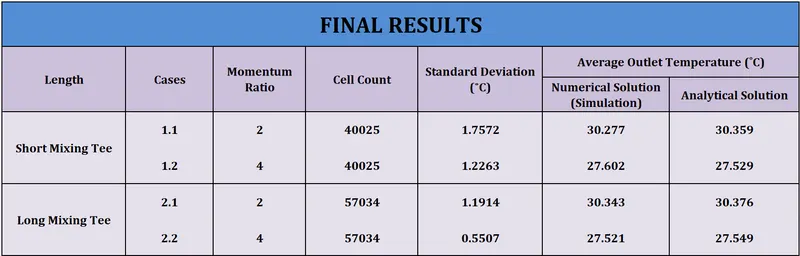
To validate the results, we compare this calculated analytical solution with the numerical (simulation) results, as shown below.
FINAL RESULTS :
The below table represents the final results of the simulation, in comparison to the analytical results.
MESH INDEPENDENCE TEST :
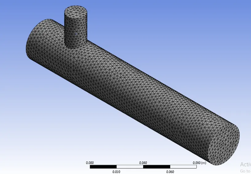
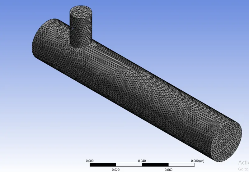
In this study, we are going to run the simulation for 3 different mesh sizes. The objective of this test is to determine whether the change in mesh size leads to a change in the output of the simulation.
We are considering 3 cases of default mesh size, 0.003 and 0.002 element sizes respectively.
Default Element Size :
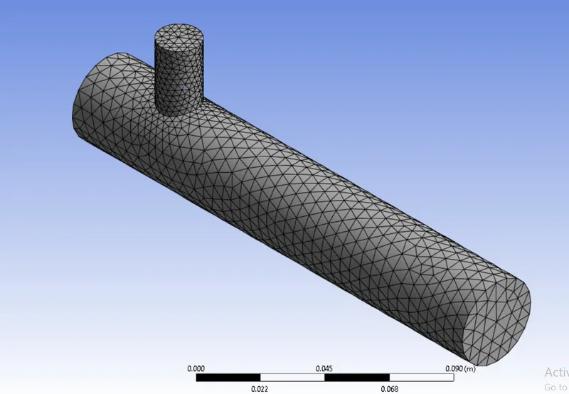
Element Size 0.003 :
Element Size 0.002 :
Results :
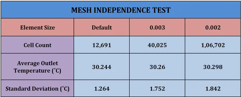
From the above table, we can observe that with the change in mesh element size, there is not much change of the average temperature at the outlet and the standard deviation, when compared to each other. Therefore, we can conclude that the simulation is mesh independent.
As the mesh size increases, the standard deviation value also rises. This is because, as the meshing size or number of cells increases, it also leads to the values being calculated more accurately. This, thereby leads to increased deviation between the cells.
CONCLUSION AND DISCUSSIONS :
- The simulation to represent the fluid flow through a mixing tee has been successfully carried out for a short & long mixing tees and the general contour plots of temperature and velocity along with its residual plots, area weighted average and standard deviation plots have been obtained for all the 4 sub-cases.
- From the comparison study, we have opted to use the realizable k-ɛ turbulence model for the further cases on the basis that the k-ɛ model has lesser standard deviation, leading to more efficient mixing, when compared to the k–ω model.
- From the sub-case study, we can observe that a higher momentum ratio value, which further leads to an increase in cold air inlet velocity, leads to much more efficient cooling when compared to a lower momentum ratio value. Therefore, increasing the cold inlet velocity leads to more efficient cooling.
- Similarly, by increasing the length of the tee geometry, we obtain a lesser standard deviation value. This means that, with the increase in the length of the tee geometry, the standard deviation value reduces. A low standard deviation value leads to better mixing of the fluids in study.
But the length of the tee geometry has no affect on the output temperature of the fluid, when compared to the short mixing tee, as their values are approximately near.
- From the mesh independence test, we can conclude that there is not much change of the average temperature at the outlet and the standard deviation between the 3 cases and thereby, the simulation is mesh independent. Also, as the mesh size increases, the standard deviation value also increases, leading to the values being calculated more accurately. This, thereby leads to increased deviation between the cells.
- Finally, from this simulation, we can conclude that increasing the cold inlet velocity leads to much efficient cooling and an increase in the length of the tee geometry leads to better mixing of the fluids.