Otto Cycle Using Matlab

OBJECTIVE :

To write a code that can solve otto cycle and make plots for it.

• Should contain PV diagram
• Should output thermal efficiency of the engine.

INTRODUCTION :

An otto cycle is an idealized thermodynamic cycle which helps us in understanding the theoretical limits of a particular cycle. It typically describes the functioning of a Spark Ignition (SI) piston engine.

It is a description of what happens to a mass of gas subjected to changes in pressure, volume, temperature, heat addition and heat removal and thereby giving us an idea of real world systems such as I.C engines and gas turbines.

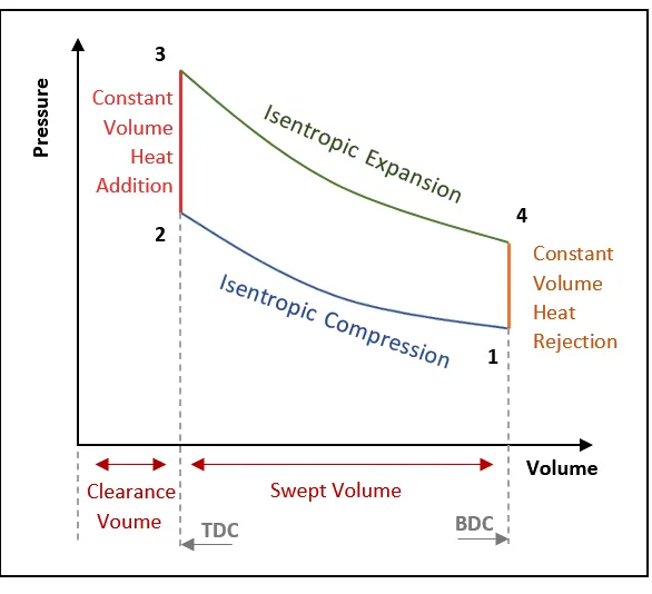
When the piston in the cylinder of Internal Combustion Engine (SI Engine) moves from BDC (Bottom Dead Centre) to TDC (Top Dead Centre), the pressure and volume relatively change, which is represented on the diagram known as PV-diagram as shown above.

The various processes involved in the above mentioned figure are as follows :

1. Process 1 – 2 : Isentropic Compression

During this process, piston moves from BDC (or crank end) to TDC (or cylinder head) and the air-fuel mixture that has entered the chamber gets compressed. The compression causes the mixture to increase in pressure from `P_1` to `P_2`, volume to reduce from `V_1` to `V_2` and temperature to increase from `T_1` to `T_2`.

2. Process 2 – 3 : Constant Volume Heat Addition

This is where combustion occurs due to ignition of fuel by spark plug. The piston in this process rests for a moment at TDC and during this time, heat is added to the working fluid by combustion of injected fuel, with the volume being held constant. Due to heat addition, the pressure increases from `P_2` to `P_3`, volume remains constant (i.e, `V_2 = V_3`) and the temperature increases from `T_2` to `T_3`.

3. Process 3 – 4 : Isentropic Expansion

The thermal energy in the chamber as a result of combustion exerts a force on piston and pushes it from TDC to BDC. This is also known as power stroke as power obtained in this process is used to do some work. Since the process involves expansion of air, the pressure decreases from `P_3` to `P_4`, volume increases from `V_3` to `V_4` and temperature falls from `T_3` to `T_4`.

4. Process 4 – 1 : Constant Volume Heat Rejection

In this process, the piston rests for a moment at BDC and rejection of heat takes place at constant volume (i.e, `V_4 = V_1`). All the waste heat is expelled from the engine chamber leading to temperature fall from `T_4` to `T_1`. As heat leaves the gas, the molecules lose kinetic energy causing a decrease in pressure from `P_4` to `P_1`.

TERMS :

1. Bore :- Bore in an engine refers to the diameter of each cylinder.
   
   
   
2. Stroke :- Stroke refers to the distance within the cylinder which the piston travels.
   
   
   

3. Compression Ratio (cr) :-

   It is the ratio of volume before compression (with the piston at BDC) to the volume after compression (with the piston at TDC). High compression ratios give increased efficiency but lead to knocking of the engine.

   `CR = (V_s+V_c)/(V_c) = (V_1)/(V_2)`
   
   

   Where, `V_1` = Volume before compression = `V_s + V_c`

   `V_2` = Volume after compression = `V_c`

   `V_s` = Swept volume

   `V_c` = Clearance volume
   
   
   
   

4. Swept Volume (Vs) :-

   Swept volume can be defined as the volume swept by the engine piston during one stroke.
   
   `V_s = (pi/4) * D² * L`
   

   Where, `D` = bore

   `L` = length of stroke
   
   
   
   

5. Clearance Volume (Vc) :-

   Clearance volume can be defined as the volume that remains in the cylinder when the engine piston is in the top dead centre position.
   
   `V_c = (V_s) / (CR – 1)`
   
   
   

6. Thermal Efficiency :-

   The thermal efficiency of any heat engine can be defined as the ratio of work done to the heat input.
   
   `eta = 1 – ( 1 / (CR^(γ-1)) )`
   

DEFINING STATE VARIABLES :

1. State point – 1 :

At state point 1, the volume of the gas or mixture is taken as V1 and the pressure at this point is taken as P1.

Assumptions :

i.) The pressure at state point 1 is assumed as 101325 Pascal, which is the atmospheric air pressure.

P1 = 101325

ii.) The temperature at state point 1 is assumed as 400K.

T1 = 400

The volume at state point 1 is taken as the sum of swept volume and clearance volume.

V1 = v_swept + v_clearance

2. State Point – 2 :

In the process, adiabatic compression of the mixture occurs as the piston moves from BDC to TDC. In this process, the piston does work on the gas. As it is an isentropic (adiabatic) compression process,

The volume at this state point is equal to clearance volume.

V2 = v_clearance

Considering the equation, `P*V^ γ = constant`

i.e, `P1*V1^gamma = P2*V2^gamma`

`P2 = P1*((V1)/(V2))^gamma`

`P2 = P1*(cr)^gamma`

Using the ideal gas law, `(P*V)/T = constant`

i.e, `(P1*V1)/(T1) = (P2*V2)/(T2)`

`T2 = (P2*V2*T1)/(P1*V1)`

Where,

P2 = pressure at state 2

V2 = volume at state 2

T2 = temperature at state point 2

`gamma = (Cp)/(Cv)`

`(V1)/(V2) = compression ratio (cr)`

3. State Point – 3 :

This process is a constant volume heat addition to the working gas when the piston is at TDC. The process represents the ignition of the air-fuel mixture and its rapid burning. As heat is transferred into the system during this process, it is isochoric. There is no change in volume during heat addition or combustion.

Therefore, V3 = V2

The temperature at this point is assumed to be 2300K, which is the temperature after heat addition.

T3 = 2300

And using ideal gas law,

`(P2*V2)/(T2) = (P3*V3)/(T3)`

i.e, `P3 = (P2*T3)/(T2)`

Where, V3 = volume at state point 3

P3 = pressure at state point 3

T3 = temperature at state point 3

4. State Point – 4 :

During the process, the combustion process exerts a force on the piston and pushes it towards BDC. This is also called a power stroke as work is done on the piston when the thermal energy is turned into motion to power the vehicle or machine. At which point, the resulting volume is same as the volume of state 1.

Therefore, V4 = V1

Considering the equation, `P*V^ γ = constant`

i.e, `P3*V3^gamma = P4*V4^gamma`

`P4 = P3*((V3)/(V4))^gamma`

Where, V4 = volume at state point 4

P4 = pressure at state point 4

Thereby, the state parameters at all 4 points of the cycle have been calculated and a P-V graph can be plotted with the same.

DETAILED PROCEDURE AND EXPLANATION :

The various steps involved in writing a code to solve otto cycle are as follows.

Step – 1

The first and foremost thing is to find out how the volume changes from state-1 to state-2. That is nothing but finding out the volume trace.

The volume trace depends on the engine kinematics and hence we need to define the engine geometric parameters first.

The engine geometric parameters are as follows:-

i.) Bore

ii.) Stroke length

iii.) Connecting rod length

iv.) Compression ratio ( cr ).

Code:

% engine geometric parameters
bore = 0.25
stroke = 0.1
connecting_rod = 0.15
cr = 13

Once we have these equations, we can calculate the swept volume and clearance volume, which is the information needed to calculate V1 and V2.

Step-2

The next step involves the calculation of swept volume and clearance volume.

We know, swept volume is the volume of cylinder defined by bore and stroke.

Therefore, Swept Volume = `(pi/4) * D² * L` where, D = bore

L = stroke length

Clearance volume is the volume remaining above the piston of IC engine when it reaches TDC.

Therefore, Clearance volume = `(Vs) / (cr – 1)` where, Vs = swept volume

cr = compression ratio

Code:

% swept and clearance volume
v_swept = (pi/4)*bore^2*stroke
v_clearance = v_swept/(cr-1)

And also,

Total Volume, V1 = swept volume + clearance volume

And V2 = volume at TDC = clearance volume

Code:

% total volume
v1 = v_swept + v_clearance
v2 = v_clearance

Step-3

The next step in the coding process is the input of assumed values and state point variables at each of the four points, into the program. As we have previously calculated the state point variables, by using governing equations and ideal gas laws,

Code:

% inputs
gamma = 1.4
t3 = 2300

% stage 1
p1 = 101325
t1 = 400

% stage 2
% p1v1^gamma = p2v2^gamma   /   p2 = p1*(v1/v2)^gamma
p2 = p1*(v1/v2)^gamma

% p1v1/t1 = p2v2/t2   /   t2 = p2*v2*t1/(p1*v1)
t2 = p2*v2*t1/(p1*v1)

% stage 3
v3 = v2

% p2v2/t2 = p3v3/t3   /   p3 = p2*t3/t2
p3 = p2*t3/t2

% stage 4
v4 = v1

% p3v3^gamma = p4v4^gamma
p4 = p3*(v3/v4)^gamma

From the above code, we thereby compute the variables at state points 1, 2, 3 and 4 respectively. With the help of these points, we can thereby plot the co-ordinates of the state points on the PV graph.

Code:

% plotting
hold on
plot(v1,p1,'*','color','r')
plot(v2,p2,'*','color','r')
plot(v3,p3,'*','color','r')
plot(v4,p4,'*','color','r')
title('Otto cycle using Matlab')
xlabel('Volume (m³)')
ylabel('Pressure (Pa)')

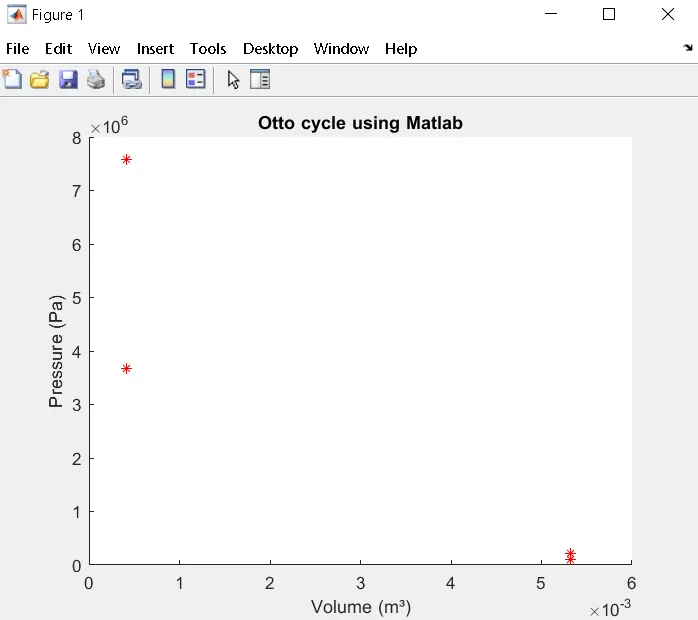
The above code plots the state point variables on the PV graph.

Output plot:

Step-4

Before solving the otto cycle program, we first need to solve the Piston Kinematics Equation. This equation tells us how the piston moves from TDC to BDC and how the combustion chamber volume changes as a function of crank angle.

The relation determining how volume inside the combustion chamber is going to change is given by,

`V/(Vc) = 1 + 1/2*(cr – 1)*[R + 1 – costheta – (R^2 – sin^2theta)^(1/2)]`

Where, Vc = clearance volume

cr = compression ratio

R = connecting rod length / a

a = stroke / 2

Thereby, solving the above equation as a function of bore, stroke, connecting rod length, compression ratio, start and end crank angles, we obtain the piston kinematics equation, as a function.

Code:

function V = piston_kinematics(bore,stroke,connecting_rod,cr,start_crank,end_crank)

% inputs
theta = linspace(start_crank,end_crank,100)

% engine parameters
a = stroke/2
R = connecting_rod/a

% swept and clearance volume
v_swept = (pi/4)*bore^2*stroke
v_clearance = v_swept/(cr-1)

% equation
term1 = 0.5*(cr-1)
term2 = R + 1 - cosd(theta)
term3 = (R^2 - sind(theta).^2).^0.5

V = (1 + term1*(term2-term3))*v_clearance

end

The above equation represents the piston kinematics equation as a function, which is further used to solve the otto cycle program.

Step-5

The next step involves incorporating the above piston kinematics equation function into the main program, at the state points 2 and 3 respectively, so as to obtain the pressure and volume values of isentropic compression and expansion.

i.e, Obtaining the values of V_compression, P_compression, V_expansion and P_expansion and thereby plotting a graph for the same.

Code:

% compression parameters
constant_c = p1*v1^gamma
V_compression = piston_kinematics(bore,stroke,connecting_rod,cr,180,0)
P_compression = constant_c./(V_compression.^gamma)


% expansion parameters
constant_c = p3*v3^gamma
V_expansion = piston_kinematics(bore,stroke,connecting_rod,cr,0,180)
P_expansion = constant_c./(V_expansion.^gamma)

As we know, Thermal Efficiency of Otto cycle is given by

`eta = 1 – ( 1 / (cr^(γ-1)) )`

And thereby, representing the above equation in code form, we obtain the thermal efficiency.

Code:

% thermal efficiency
eta = 1 - (1/cr^(gamma-1))
efficiency_in_percent = eta*100

Step-6

As a result of all the above mentioned steps, we obtain the final program code to calculate the thermal efficiency of otto cycle and thereby plotting the PV graph for the same.

Final Program:

% otto cycle
clear all
close all
clc

% inputs
gamma = 1.4
t3 = 2300

% stage 1
p1 = 101325
t1 = 400

% engine geometric parameters
bore = 0.25
stroke = 0.1
connecting_rod = 0.15
cr = 13

% swept and clearance volume
v_swept = (pi/4)*bore^2*stroke
v_clearance = v_swept/(cr-1)

% total volume
v1 = v_swept + v_clearance
v2 = v_clearance

% stage 2
% p1v1^gamma = p2v2^gamma   /   p2 = p1*(v1/v2)^gamma
p2 = p1*(v1/v2)^gamma

% p1v1/t1 = p2v2/t2   /   t2 = p2*v2*t1/(p1*v1)
t2 = p2*v2*t1/(p1*v1)

% compression parameters
constant_c = p1*v1^gamma
V_compression = piston_kinematics(bore,stroke,connecting_rod,cr,180,0)
P_compression = constant_c./(V_compression.^gamma)


% stage 3
v3 = v2

% p2v2/t2 = p3v3/t3   /   p3 = p2*t3/t2
p3 = p2*t3/t2

% expansion parameters
constant_c = p3*v3^gamma
V_expansion = piston_kinematics(bore,stroke,connecting_rod,cr,0,180)
P_expansion = constant_c./(V_expansion.^gamma)

% stage 4
v4 = v1

% p3v3^gamma = p4v4^gamma
p4 = p3*(v3/v4)^gamma

% thermal efficiency
eta = 1 - (1/cr^(gamma-1))
efficiency_in_percent = eta*100

% plotting
figure(1)
hold on
plot(v1,p1,'*','color','r')
plot(V_compression,P_compression,'LineWidth',1)
plot(v2,p2,'*','color','r')
plot(v3,p3,'*','color','r')
plot(V_expansion,P_expansion,'LineWidth',1)
plot(v4,p4,'*','color','r')
plot([v2 v3],[p2 p3],'LineWidth',1)
plot([v1 v4],[p1 p4],'LineWidth',1)
title('Otto cycle using Matlab')
xlabel('Volume  (m³)')
ylabel('Pressure  (Pa)')
who

OUTPUTS:

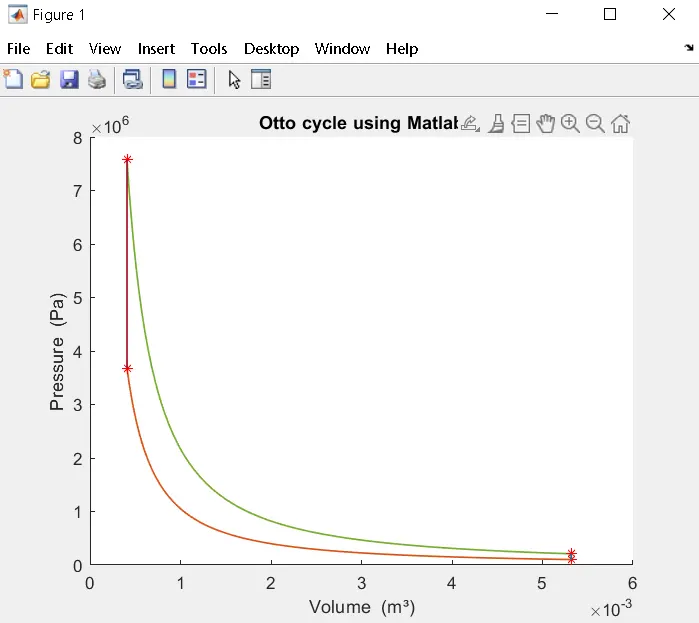
By running the above code, we obtain the PV graph of otto cycle, determining how the volume and pressure changes as a function of the various state parameters and also the thermal efficiency of the cycle.

Output Graph:

Thermal Efficiency:

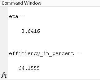
The calculated thermal efficiency is represented as shown above.

Variables:

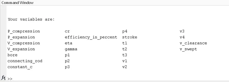
The various variables utilised in the program as displayed as follows.

PROBLEMS ENCOUNTERED:

1. While defining the piston kinematics equation function, i made a mistake of entering the function title, which was different from the file name and i got an error.

Output:

2. I entered the inputs in the wrong order, for plotting the connecting lines for the PV graph

Original:

Mistake:

Output:

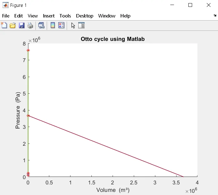
As a result of the confusion is the entry order of the above mentioned code, i obtained a wrong graph as shown above.

CONCLUSION :

1. The output PV graph has been plotted, which represents the change in pressure and volume at each state of the Otto cycle.

2. The thermal efficiency of the cycle has been calculated to be 64.15%

3. Thereby, Otto cycle has been solved using Matlab and the same approach can be employed to solve any other air standard cycle as well.