Week 10 - Simulating Combustion of Natural Gas.

AIM :

Perform a combustion simulation of natural gas, on the combustor model.

OBJECTIVES :

1. To perform a combustion simulation on the combustor model and plot the variation of mass fraction of different species in the simulation using line probes at different locations of the combustor.
   
   
   
2. Plot graphs to represent the `CO_2`, `H_2O`, `CH_4`, `N_2`, `O_2`, `NO_"x"` emissions & SOOT formation.
   
   
   
3. Add water content in the fuel from 5% to 30% by mole to observe the effect of it on the results. Provide necessary plots and contours along with the results.

INTRODUCTION :

Combustion is the process of oxidation of molecules of combustible substances that occurs readily at high temperatures with the release of energy. It is accompanied by that phenomenon which is called "flame" and by the generation of "heat energy". Combustion gas generally consists of CO₂, SO₂, O₂, N₂, and H₂O, based on complete combustion.

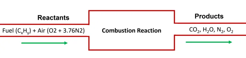
In complete combustion, the reactant burns in oxygen and produces a limited number of products. However, complete combustion is almost impossible to achieve, since the chemical equilibrium is not necessarily reached, or may contain unburnt products such as carbon monoxide, hydrogen and even carbon (soot or ash). Thus, the produced smoke is usually toxic and contains unburned or partially oxidized products.

The various types of combustion based on the mixing of fuel and air are as follows.

1. Premixed Combustion

A premixed combustion results when the fuel and oxidizer are mixed prior to the passage of the reaction zone. An example of premixed combustion is a gas stove where natural gas (70-90% methane, 30%-10% other gases) and oxygen are mixed prior to being ignited inside the burner.

2. Non - Premixed Combustion

A non-premixed flame occurs when the fuel and oxidizer are not mixed prior to reacting. An example of this is the diffusion flame from a lighter.

3. Partially - Premixed Combustion

PPC is a modern combustion process intended to be used in internal combustion engines of automobiles and other motorized vehicles in the future. Its high specific power, high fuel efficiency and low exhaust pollution have made it a promising technology. Also, the partially premixed charge burns clean.

Some examples of combustion are,

1. Burning of sulphur in the air.
2. An explosion of hydrogen in air.
3. Burning of Wax candle.
4. Combustion of petrol in a car’s engine.
5. Burning of natural gas in a bunsen burner.
6. A bush fire - means wood cellulose and other fuels burn in oxygen.

NOx Emissions :

In atmospheric chemistry, NO_x is shorthand for nitric oxide (NO) and nitrogen dioxide (NO₂), the nitrogen oxides that are most relevant for air pollution. These gases contribute to the formation of smog and acid rain, as well as affecting tropospheric ozone. NO_x gases are usually produced from the reaction between nitrogen and oxygen during combustion of fuels, such as hydrocarbons in air, especially at high temperatures, such as in car engines.

Pre-combustion method prevents `NO_"x"` from forming in the first place. Pre-combustion `NO_"x"` reduction is accomplished by either staging the combustion process or recirculating flue gases into the combustion process.

Soot Formation :

Soot is a mass of black, impure carbon particles resulting from the incomplete combustion of hydrocarbons. Soot emission from a practical combustion appliance reflects poor combustion conditions and a loss of efficiency.

Soot as an airborne contaminant in the environment has many different sources, all of which are results of some form of pyrolysis. They include soot from coal burning, internal-combustion engines, power-plant boilers, hog-fuel boilers, ship boilers, central steam-heat boilers, waste incineration, local field burning, house fires, forest fires, fireplaces, and furnaces.

Since soot is sticky, it tends to stick to exhaust pipes and chimneys where the combustion occurs. Soot in very low concentrations is capable of darkening surfaces or making particle agglomerates, such as those from ventilation systems, appear black. Soot is the primary cause of "ghosting", the discoloration of walls and ceilings or walls and flooring where they meet.

Turbulent Chemistry Interaction (TCI) models :

The turbulence chemistry interaction model with finite rate chemistry is a common model for solving supersonic turbulent combustion and takes into consideration the interaction between turbulent mixing and chemical reactions as well as finite chemistry reaction. Considering engineering applications, the compressibility correction was introduced to two recent turbulence chemistry interaction models with finiterate chemistry, the Partially Stirred Reactor (PaSR) model and Unsteady PaSR (UPaSR) model, in a Reynolds Averaged Navier Stokes (RANS) framework.

Numerical simulations of two typical supersonic combustors showed that the interaction between the turbulence and combustion was intensive with complex supersonic chemical reaction flow and could be described by the fine scale structure volume fraction. The distributions of temperature, pressure, velocity and components somewhat downstream of fuel injection areas were most obviously improved by the presented models. Moreover, the increase in computational time consumption by the compressibility correction was less than 2%.

One such TCI model is the Eddy Dissipation Model.

The Eddy Dissipation model provides an empirical expression for the mean reaction rate based on the assumption that chemical reaction occurs in the regions where the dissipation of turbulence energy takes place. In flows of moderate to intensive turbulence, these areas are concentrated in isolated regions, occupying only a small fraction of the flow.

SIMULATION PROCEDURE :

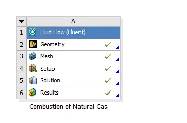
In this challenge, we are going to carry out the simulation in 5 major steps, namely.

1. Geometry
2. Meshing
3. Setup
4. Solution
5. Results

1. GEOMETRY

The first and foremost step in geometry setup is importing the step file model into the ANSYS SpaceClaim software. The imported geometry is as shown.

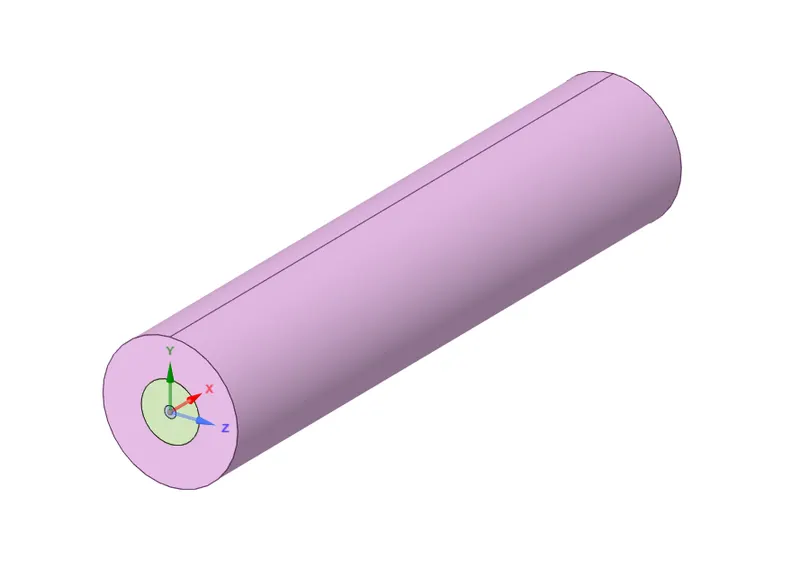
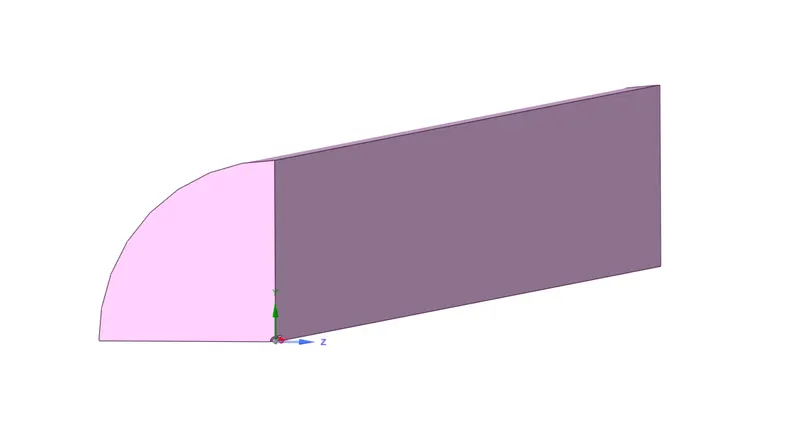
In the next step, we consider the geometry to be axi–symmetric and we obtain a cut – body view of the geometry along the X-Y plane, representing the half split geometry, as the simulation of the whole geometry would be very time consuming. We split it in half once again along the X-Z plane, so as to obtain the quarter section of the entire geometry.

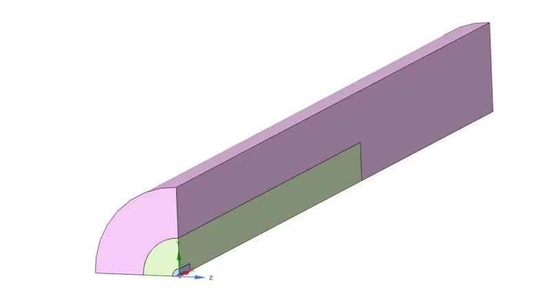
We thereby combine all the three components of the geometry using the ‘combine’ function in the design tab, so as to obtain a single plain surface out of which we can extract a 2-D geometry surface. We thereby obtain the wedge geometry as follows.

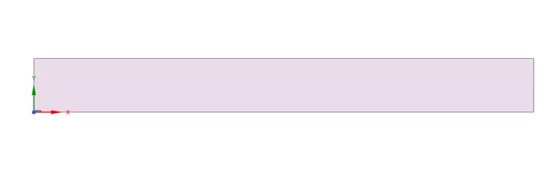
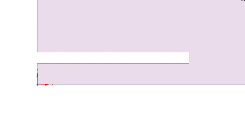
Finally, we copy the geometry surface and we paste it onto a new design plane and thereby, obtaining the final 2D surface of the combustor. We make sure to close the 3D geometry before moving on to the meshing step.

2. MESHING

Before generating the mesh for the 2D surface, we first create the named selections for the various surfaces of the geometry as follows.

A.) Fuel Inlet – from where the fuel enters the combustor.

B.) Air Inlet - from where the air enters the combustor.

C.) Axis – axi-symmetric axis of the surface.

D.) Outlet – through which the gas mixture exits the combustor.

E.) Walls – stationary wall enclosing the combustor chamber.

F.) Interior Walls.

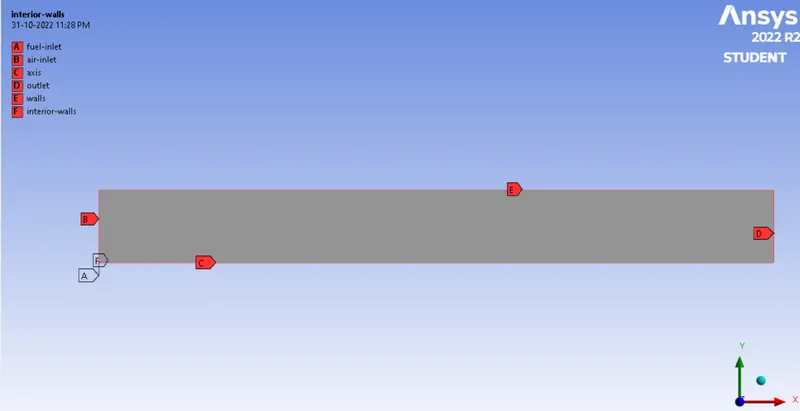
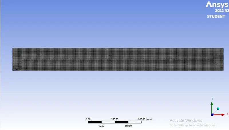
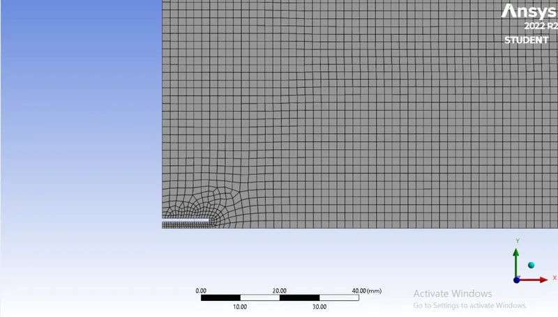
Next, we generate a quadrilateral dominant mesh (which is generated by default for the 2D surface) of an element size of 2 mm, for the 2D surface. Also, we capture the proximity so as to obtain finer meshing around the combustor fuel inlet. The final meshed geometry is as shown.

3. SETUP

The general setup conditions are the same for all the cases and are as follows.

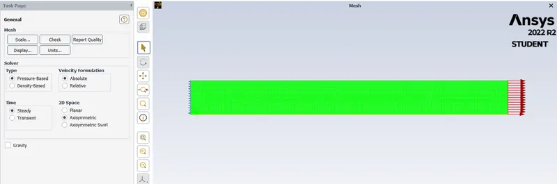
• For the setup of this simulation, we use a pressure based solver with absolute velocity formulation, operating at a steady state condition.
  
  
• As we have considered the geometry to be axi-symmetric, we set the 2D space to axi-symmetric as well.
  
  
• We enable the energy equation as we are involving the calculations of temperatures in our simulation.

Turbulence Model :

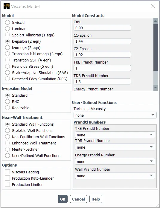
In this simulation, with relevance to the Reynold’s number of the flow and also, as we are using the Eddy Dissipation model further on, we need to choose a turbulence model, as the Eddy Dissipation model is a Turbulent Chemistry Interaction (TCI) model. Thereby, we select the standard k – epsilon turbulence model with standard wall functions to run the simulation.

Species Model :

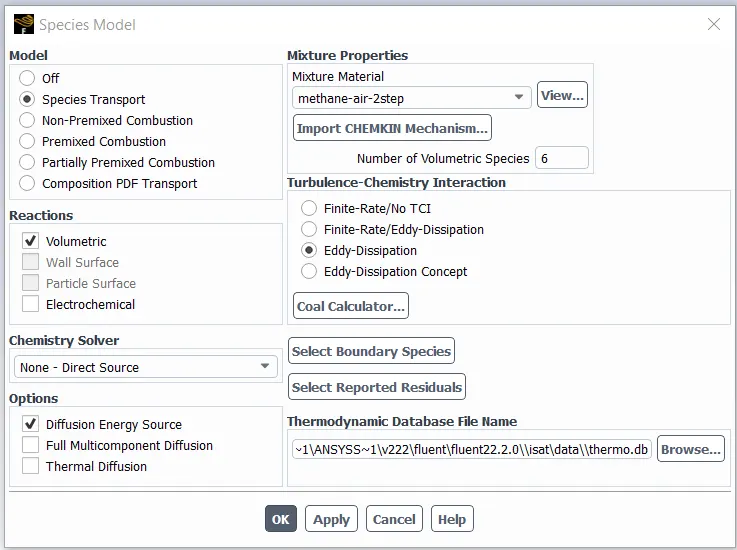
The species model in ANSYS Fluent is used to model the mixing and transport of chemical species by solving conservation equations describing convection, diffusion and reaction sources for each component species. In this step, we set the parameters related to the calculation of species transport and combustion.

• Convection, diffusion, and reaction sources conservation equations for many component species are solved using the species transport method, being used in this simulation.
  
  
  
• We enable the volumetric reactions as they are taking place in a gas phase.
  
  
  
• We use methane-air-2step as the mixture material, as it allows the addition of water to fuel or air.
  
  
  
• To avoid costly chemical kinetic calculations, reaction rates are believed to be controlled by turbulence while neglecting the impact of chemistry timeframes in the Eddy Dissipation TCI model. The model is computationally cheap, but only one or two-step heat-release mechanisms should be utilized for realistic results.

`NO_"x"` Model :

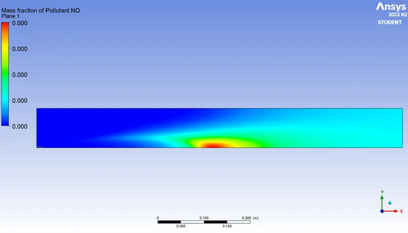
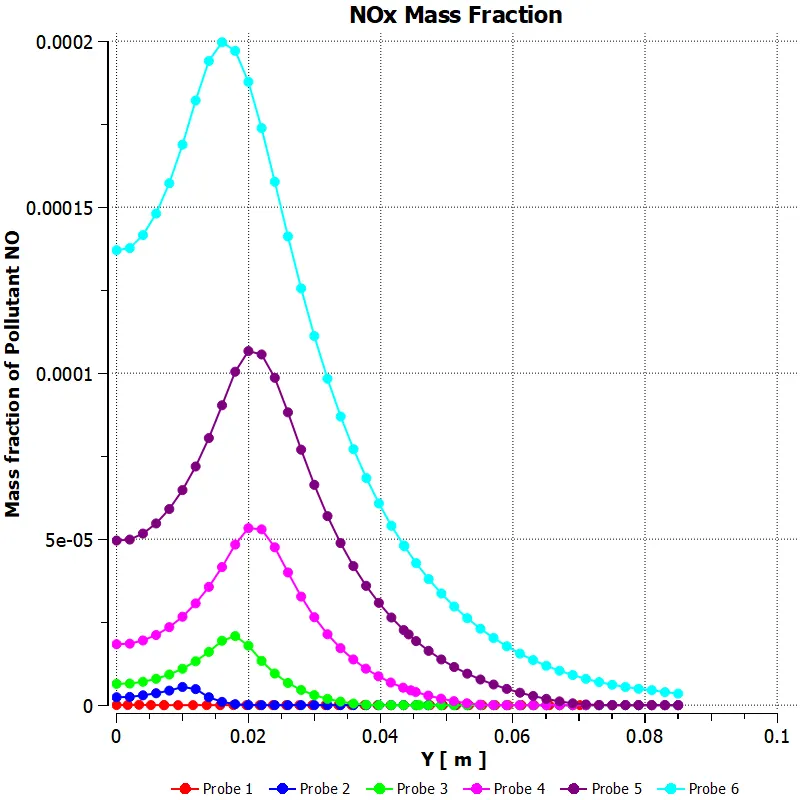
The formation of `NO_"x"` occurs during combustion due to rich fuel mixtures and high temperatures. In order to track the pathways of generation of `NO_"x"` during the combustion process, we activate the `NO_"x"` model.

There are four different mechanisms to form `NO_"x"`: Thermal, Prompt, Fuel and N₂O route.

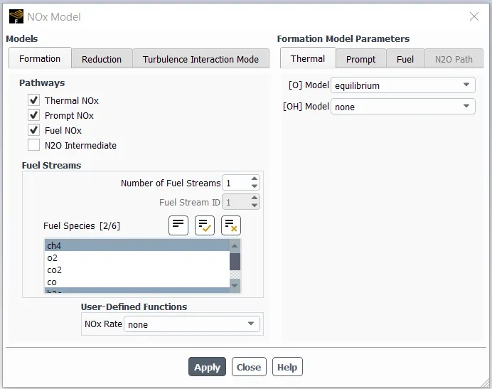
We track the NOx emissions for `CH_4` and `H_2O` species as they are the components undergoing combustion in the combustor.

Soot Model :

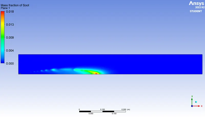
Soot particles are generally formed due to incomplete combustion or pyrolysis in rich mixture of hydrocarbon fuel with strong temperature gradients in combustion chamber. In order to track this, we activate the one – step soot model as follows.

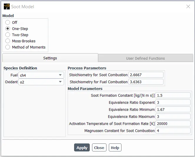
The fuel in the case of this simulation is considered as CH4 (methane 2-step) and the oxidant is considered to be air.

We make sure the cell zone condition of the combustor surface is set to methane-air-2step and we further move on to providing the initial and boundary conditions for the simulation. The fuel inlet boundary conditions vary from case to case as we are varying the mass fractions of the species whereas the air inlet conditions remain constant for all the cases.

Boundary Conditions :

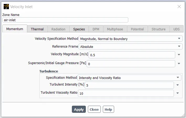
1. Air Inlet (Velocity inlet)

The air enters the combustor at an initial velocity of 0.5 m/s and an ambient temperature of 300K. The air inlet conditions are defined as follows.

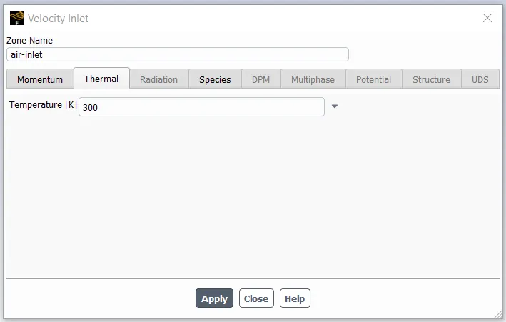
The reaction which we are assuming to take place is,

`CH_4 + a_r ( O_2 + 3.76N_2) -> CO_2 + bH_2O + cN_2`

The above equation represents a stoichiometric equation and thereby, performing element balance on the left and right hand sides of the equation as follows.

1. Carbon Balance

`1 = a`

2. Hydrogen Balance

`4 = 2b`

3. Oxygen Balance

`2a_r = 2a + b`

`a_r = a + b/2`

Therefore, `a_r = 2` (number of moles)

From our reaction equation we have,

`a_r ( O_2 + 3.76N_2)`

`2 xx ( O_2 + 3.76N_2)`

Therefore, `2` `"moles of"` `O_2` `+` `7.52` `"moles of"` `N_2`

As we know,

`"Mole Fraction" = "Number of Moles of Species" / "Total Number of Moles"`

`"Mole Fraction of"` `O_2 = 2 / 9.52 = 0.21`

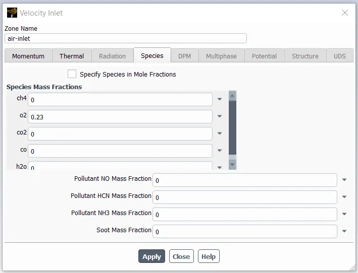
Converting the mole fraction value to mass fraction, we get the mass fraction value of `O_2` as `0.23`. Thereby, we substitute this mass fraction value of `O_2` at the air inlet as shown.

2. Fuel Inlet (Velocity Inlet)

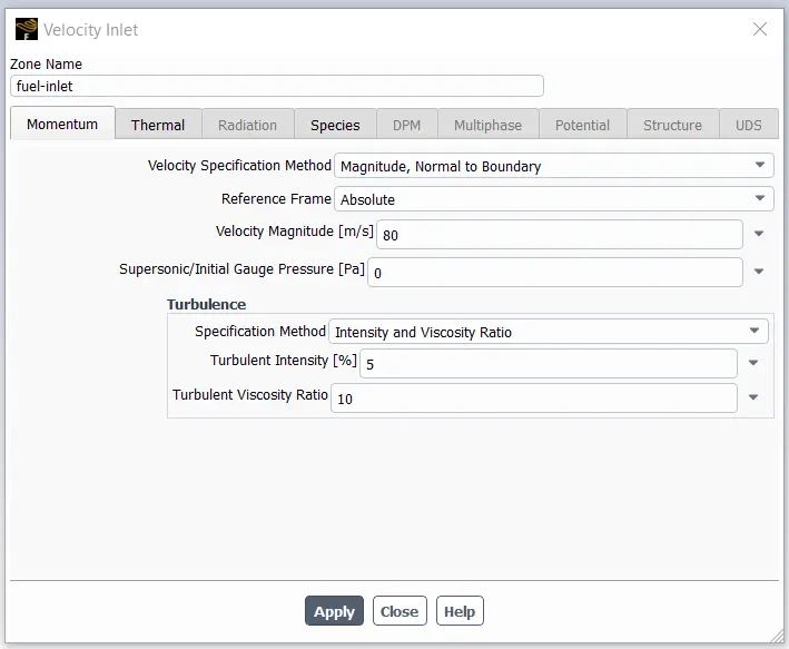
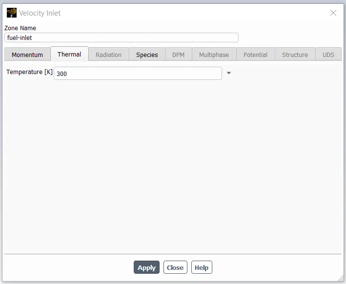
The velocity of the fluid at the fuel inlet is taken as 80 m/s at 300K temperature. The species conditions of the fuel inlet differ with respect to each case study.

3. The combustor outlet is provided with a pressure outlet boundary condition at 0 gauge pressure.

4. The walls of the geometry are considered to be stationary with a no-slip shear condition.

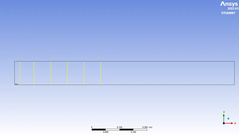
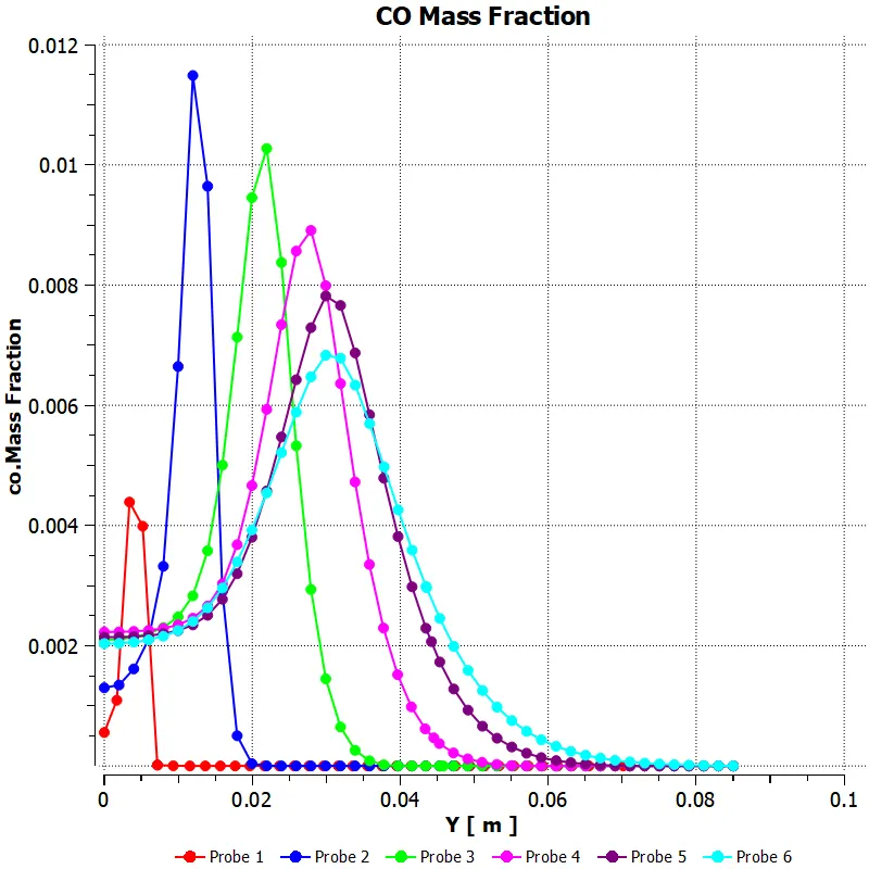
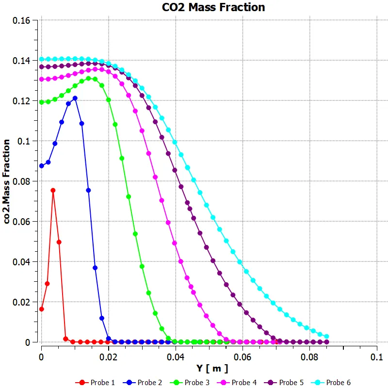
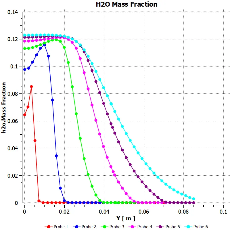
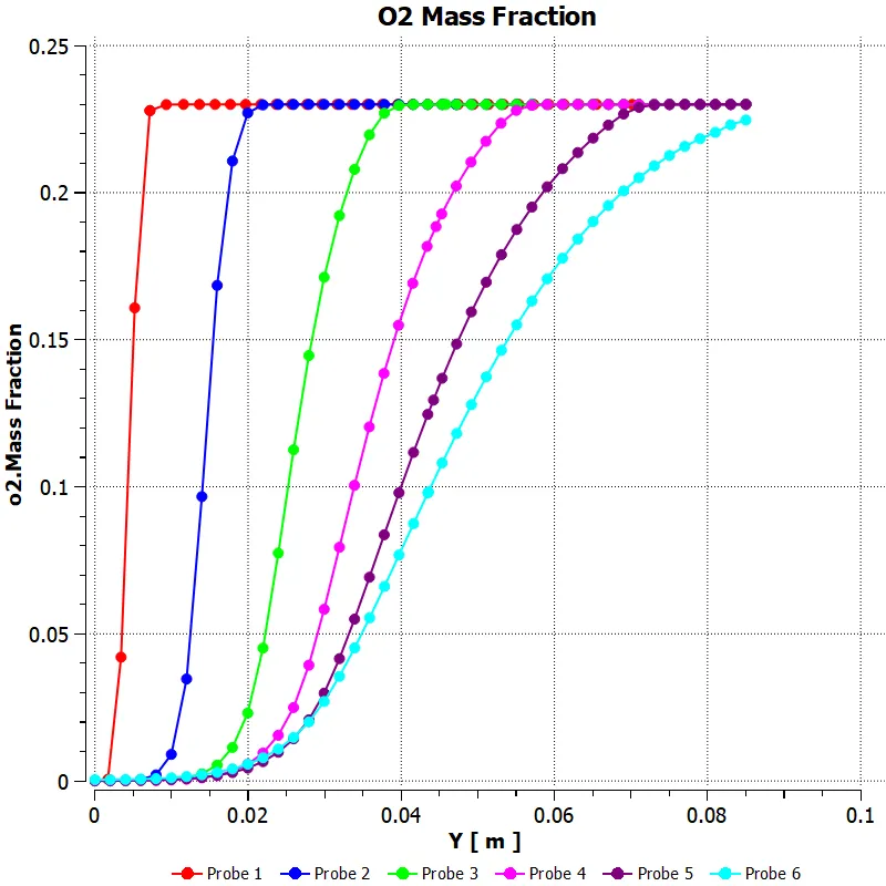
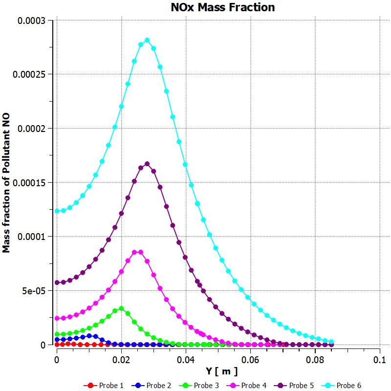
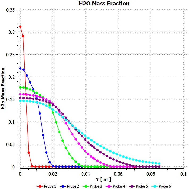
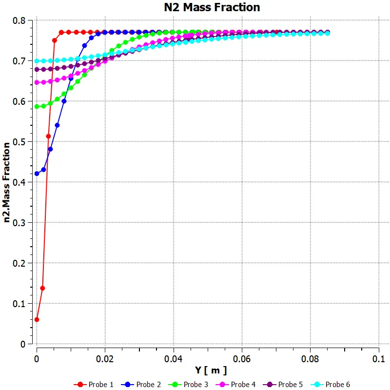
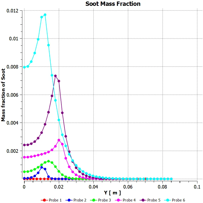
Finally, we draw 6 line probes across the combustor geometry with the help of which, we plot the variation in mass fractions of `CO_2`, `H_2O`, `CH_4`, `N_2`, `O_2` as well as `NO_"x"` emissions & Soot formation.

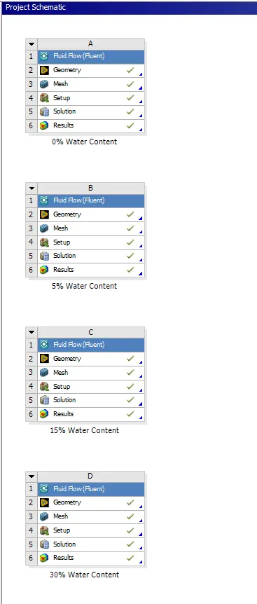
In this challenge, we run the simulation for 3 case studies – representing the addition of water content in the fuel mixture, ranging from 5% to 30% by mole, so as to observe its effects on the results and emissions. We first run a case with no water content in the fuel mixture so as to observe the differences in results obtained.

CASE – 1 : 0% WATER CONTENT

In this case setup, with reference to the general setup of the simulation, the boundary conditions of the fuel inlet in terms of species mole fractions are as shown.

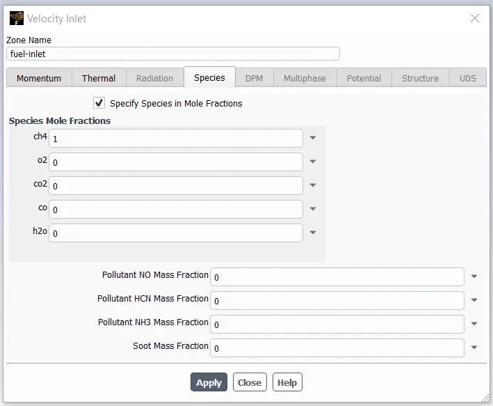
Mole Fraction of `CH_4` `= 1` (as we have only `CH_4` coming in)

Mole Fraction of `H_2O` `= 0` (no addition of water)

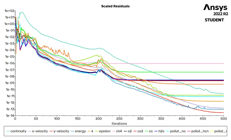
We hybrid initialize the solution and run it for 500 iterations to obtain the following results and plots.

Residuals Plot :

Temperature Plot (Contour & Chart) :

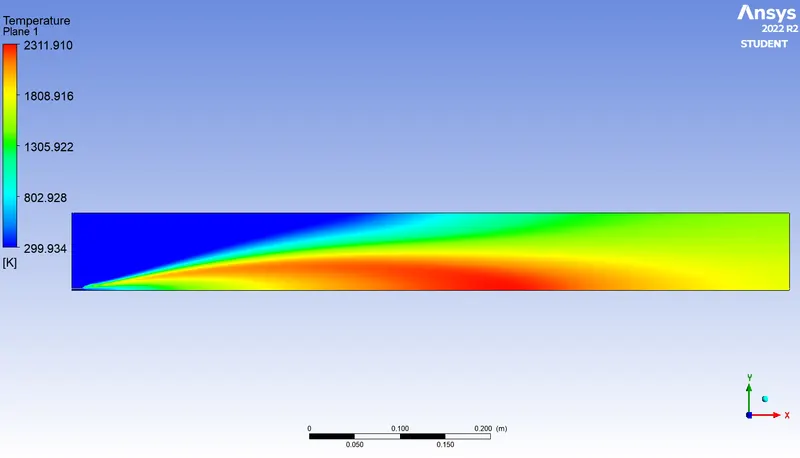
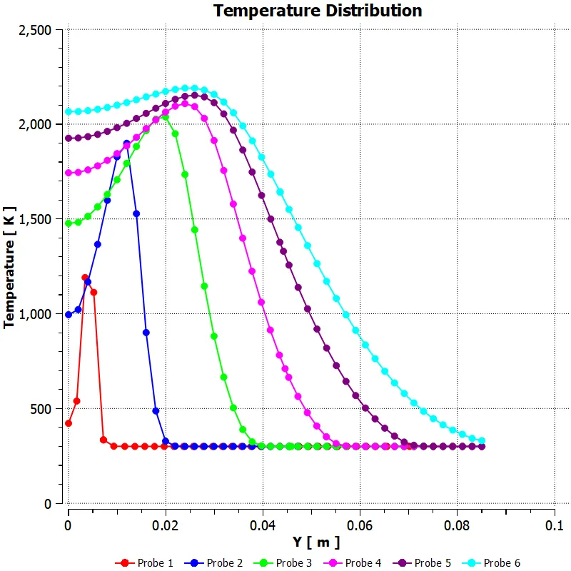
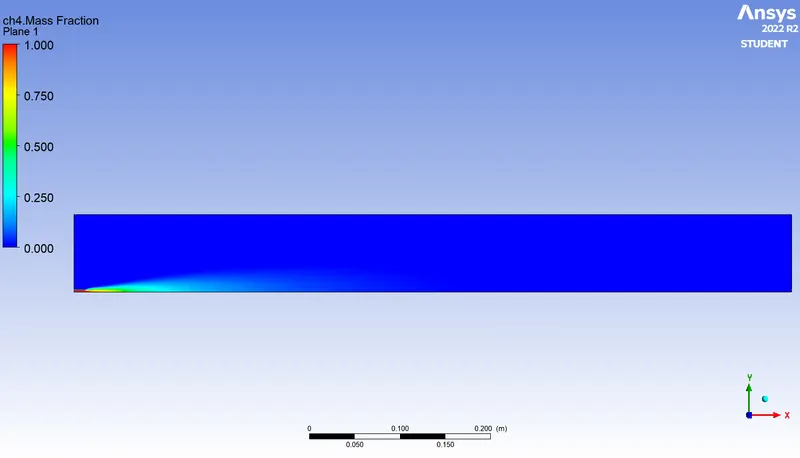
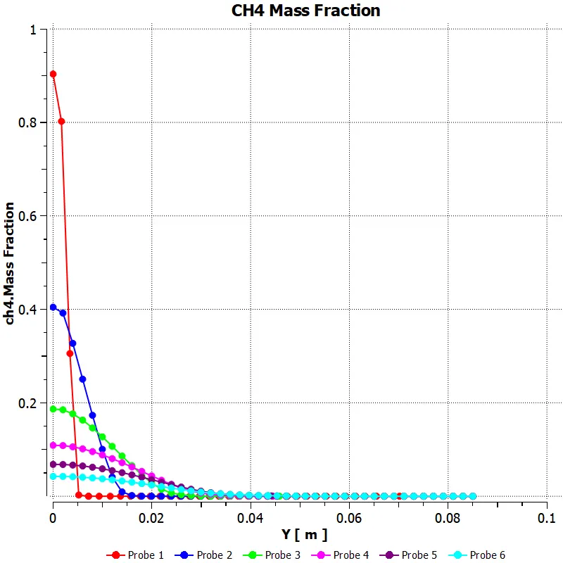
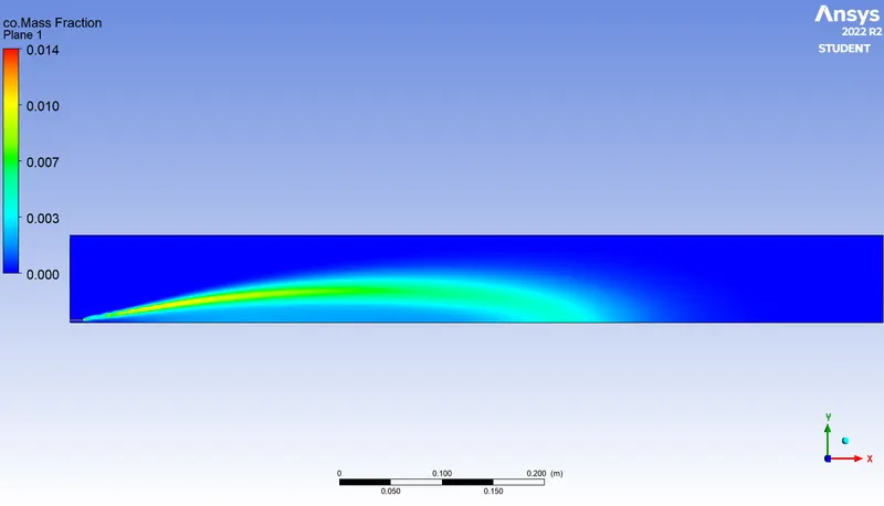
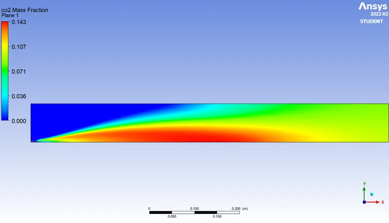
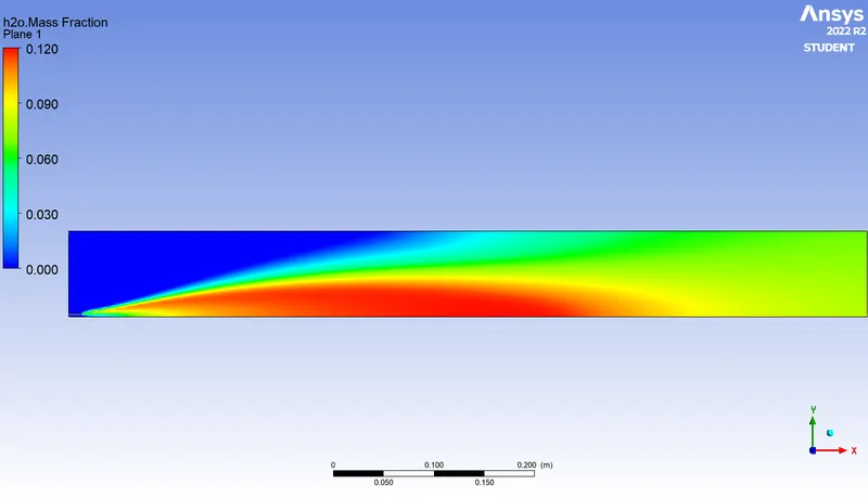
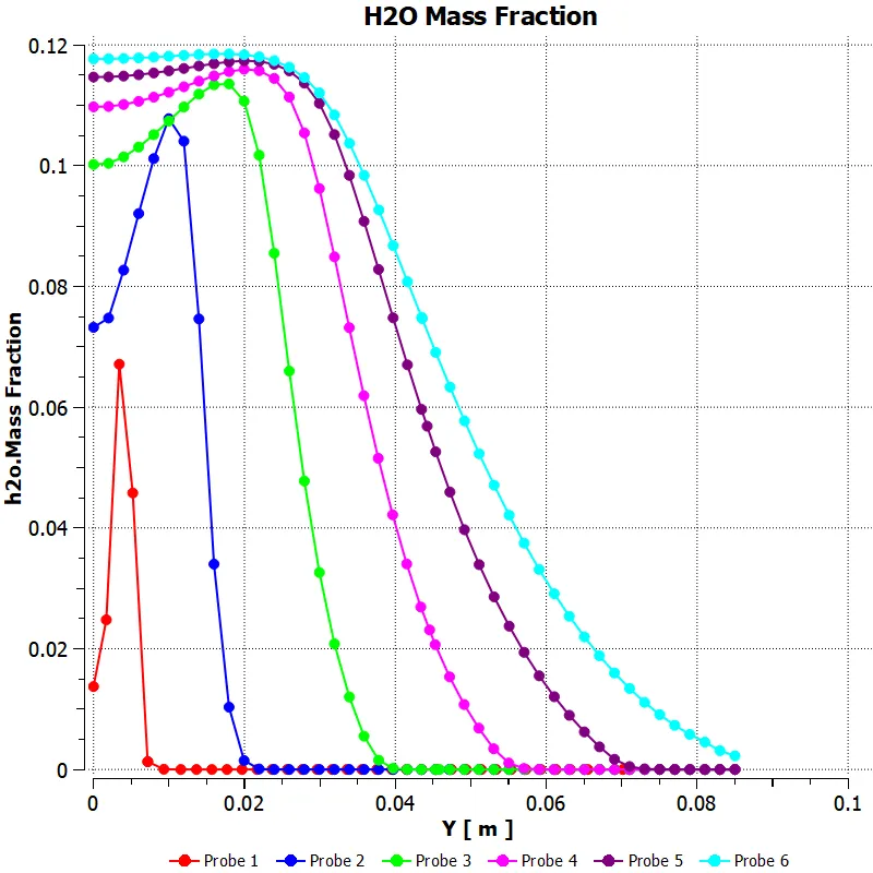
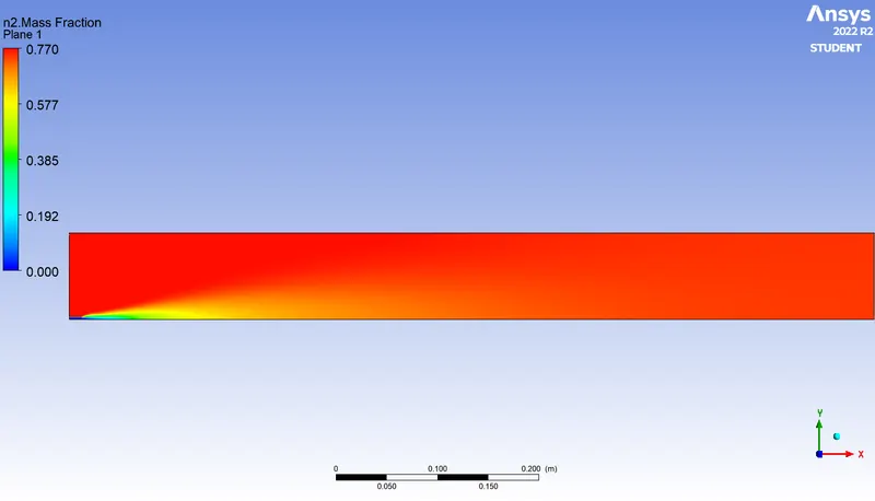
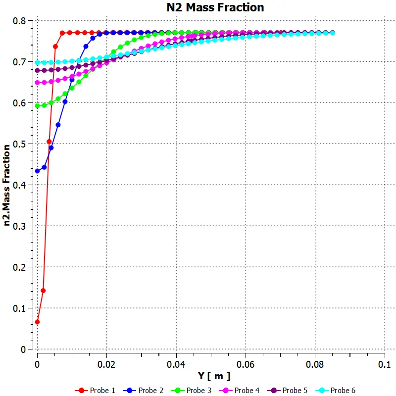
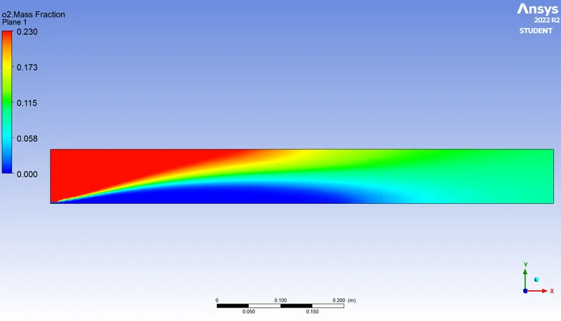
Mass Fractions of Species (Contour & Charts) :

`1.` `CH_4`

`2.` `CO`

`3.` `CO_2`

`4.` `H_2O`

`5.` `N_2`

`6.` `O_2`

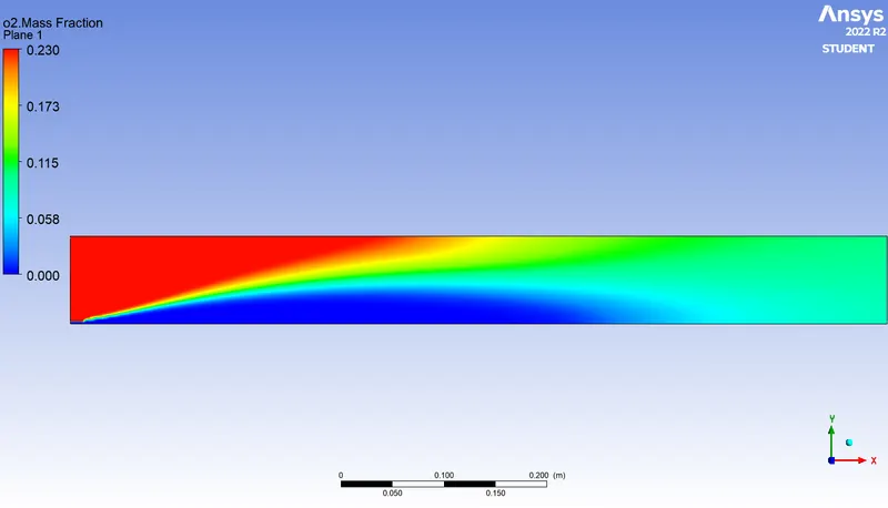
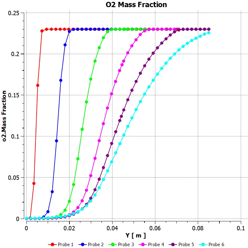
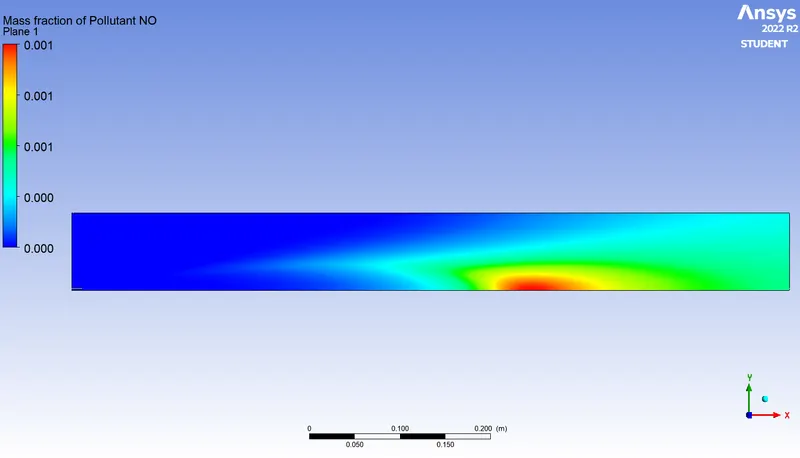
`NO_"x"` Emissions :

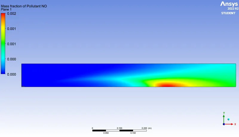
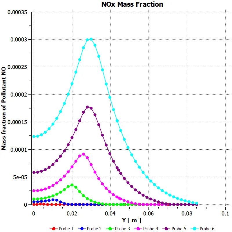
Soot Formation :

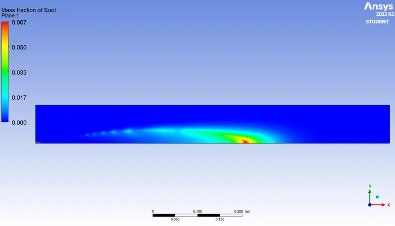
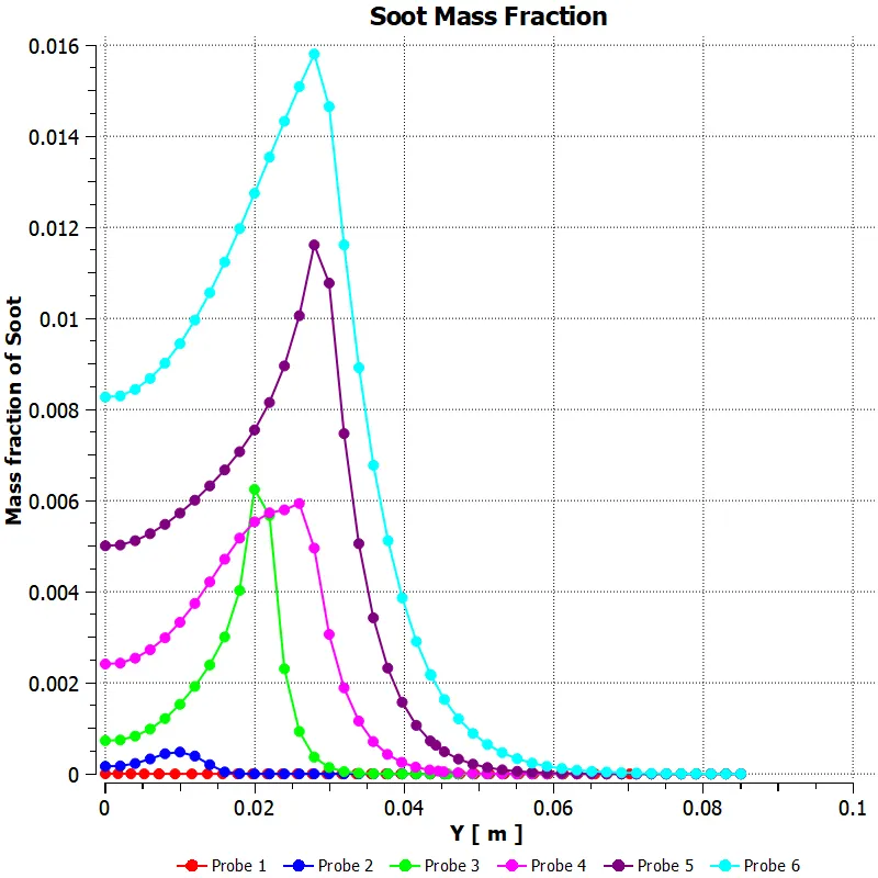
CASE – 2 : 5% WATER CONTENT

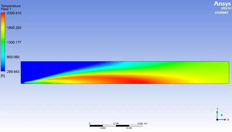
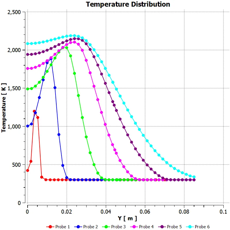
In this case setup, we consider 5% of water content mixed with the fuel, so as to observe its effects on NOx and Soot formations.

The water content is specified in terms of mole fraction at the fuel inlet as follows.

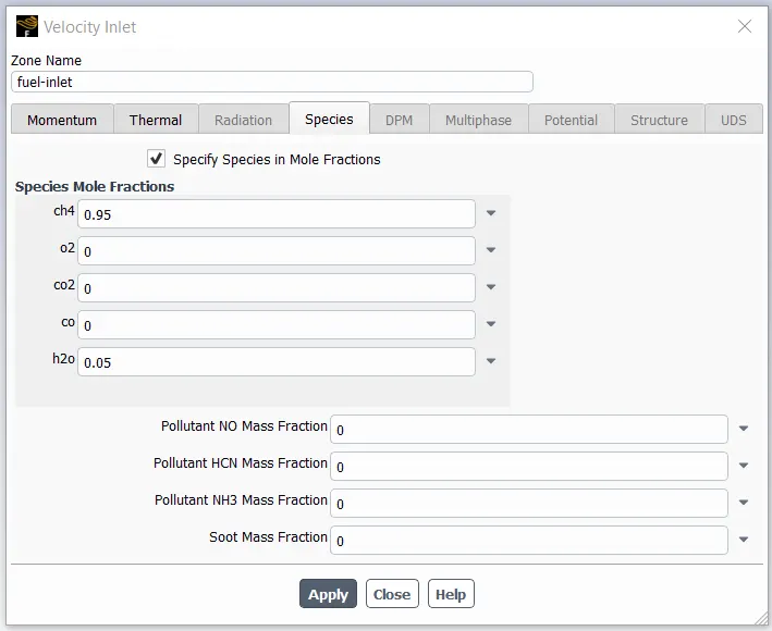
Mole Fraction of `CH_4` `= 0.95` (`95%` fuel)

Mole Fraction of `H_2O` `= 0.05` (`5%` water)

We hybrid initialize the solution and run it for 500 iterations to obtain the following results and plots.

Residuals Plot :

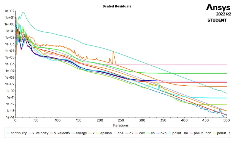
Temperature Plot (Contour & Chart) :

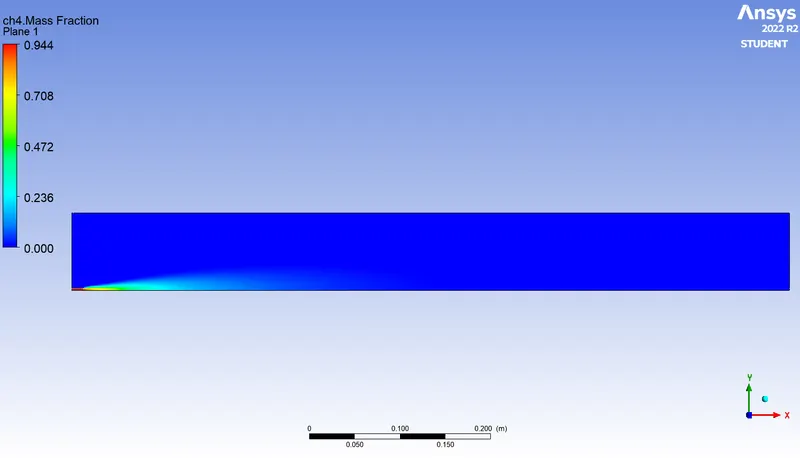
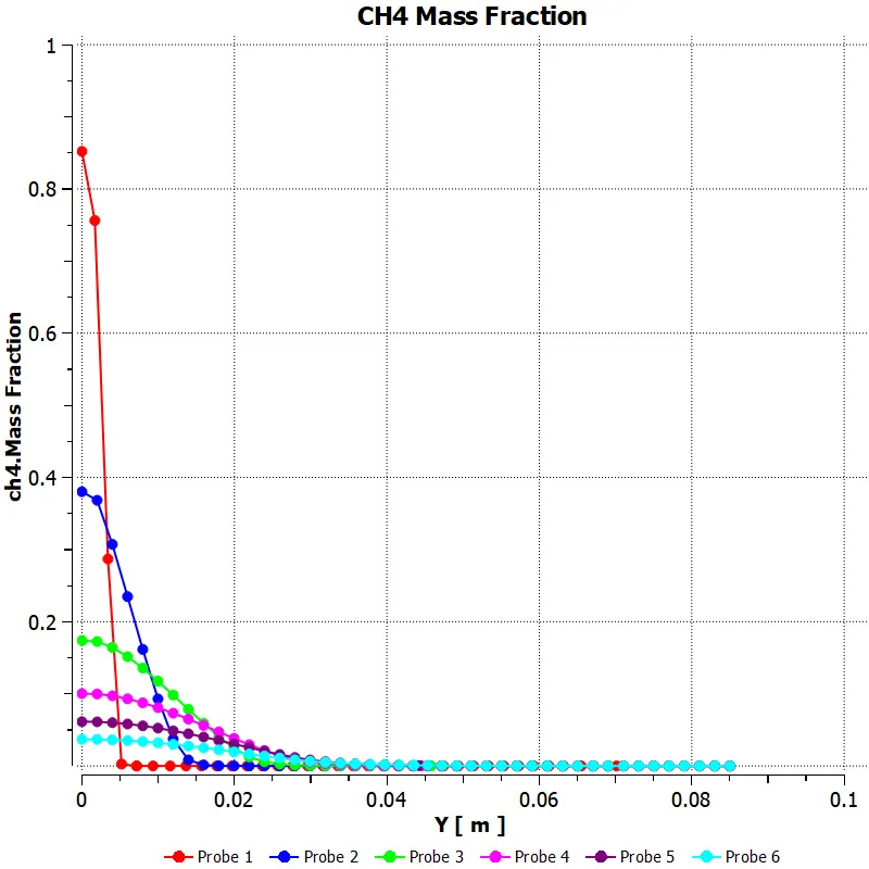
Mass Fractions of Species (Contour & Charts) :

`1.` `CH_4`

`2.` `CO`

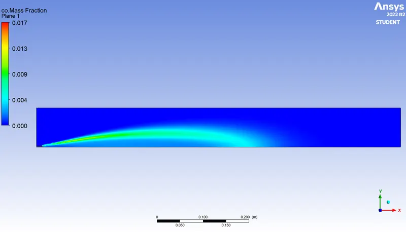
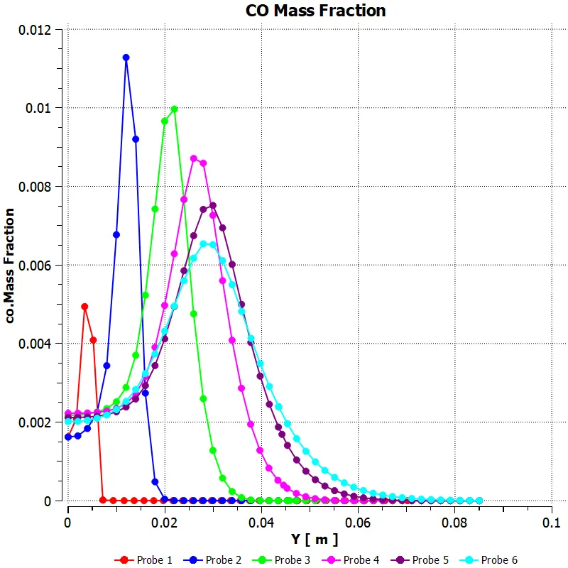
`3.` `CO_2`

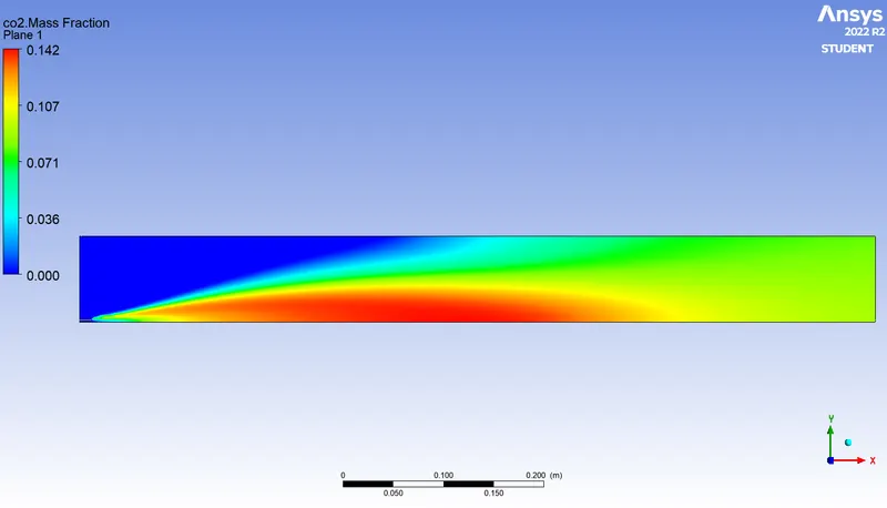
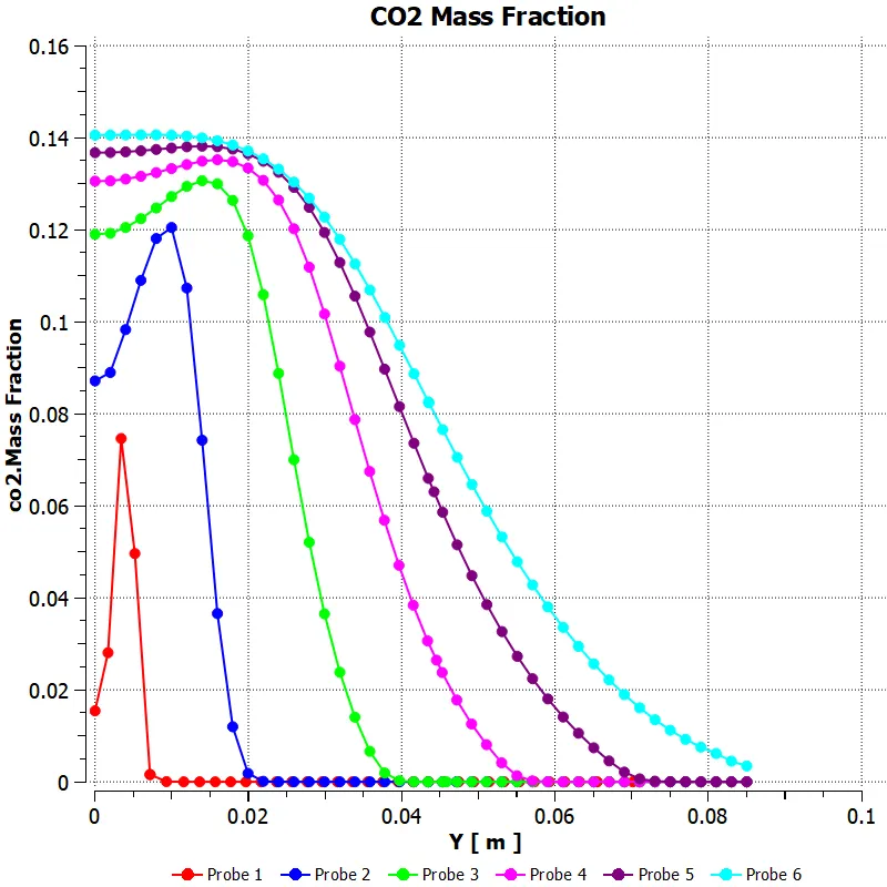
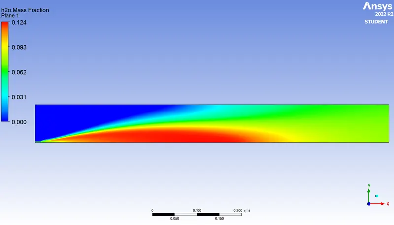
`4.` `H_2O`

`5.` `N_2`

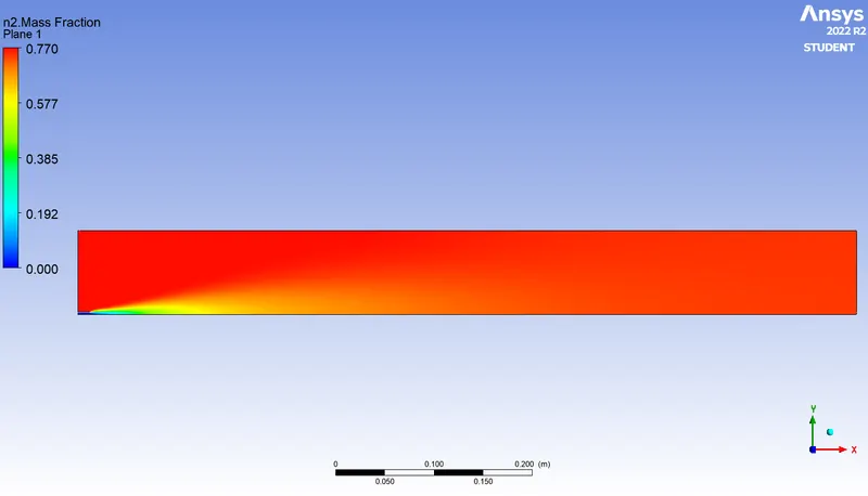
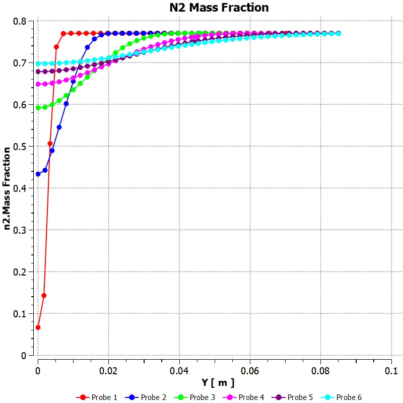
`6.` `O_2`

`NO_"x"` Emissions :

Soot Formation :

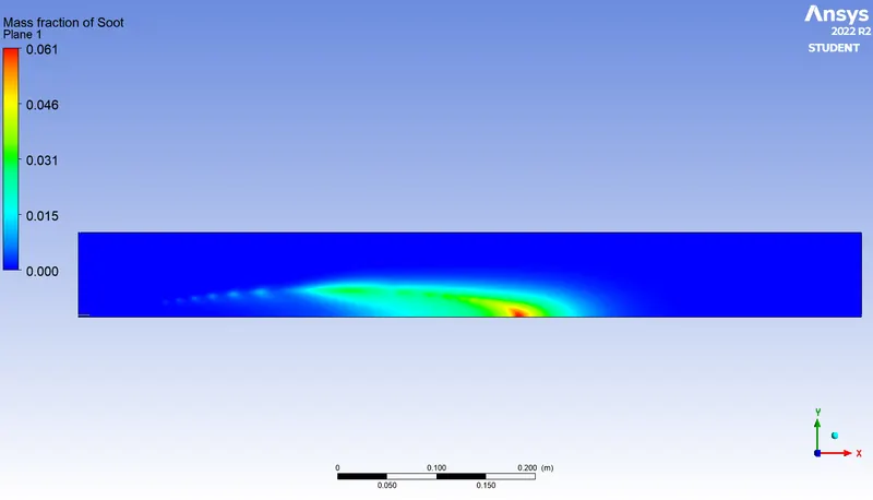
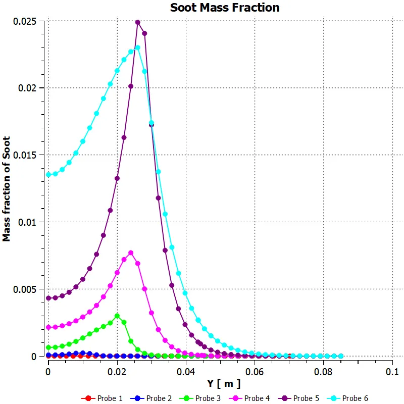
CASE – 3 : 15% WATER CONTENT

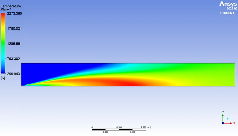
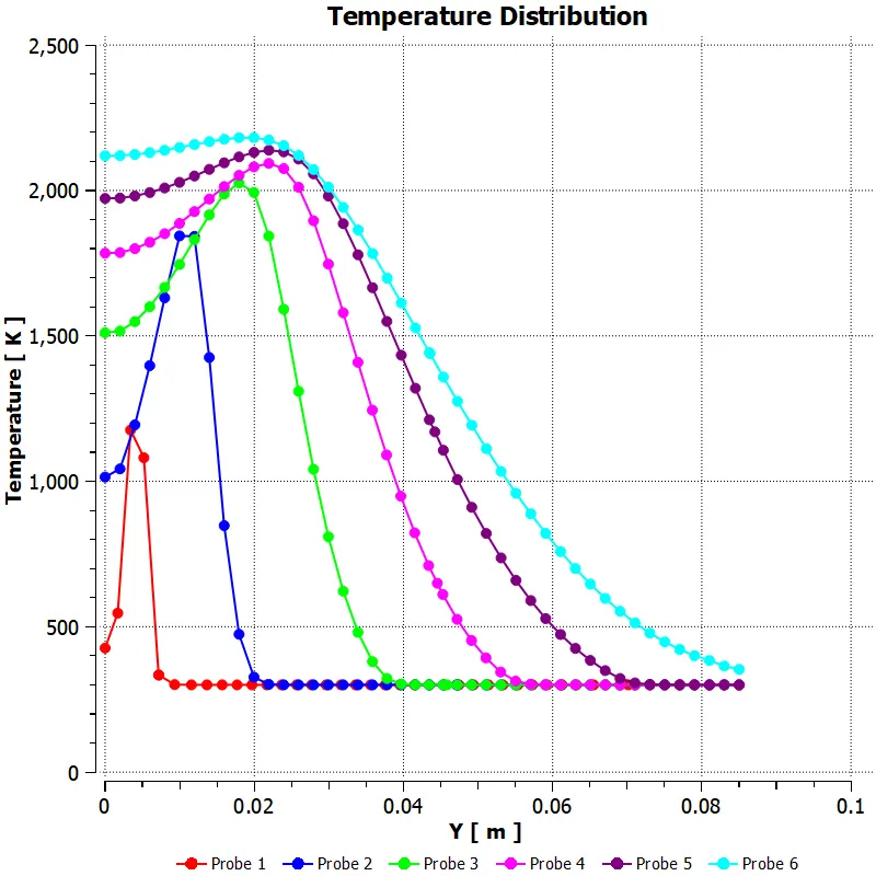
In this case setup, we increase the water content in the fuel mixture to 15% and we run the simulation to study the effects of this increased water content on the results.

The water content is specified in terms of mole fraction at the fuel inlet as follows.

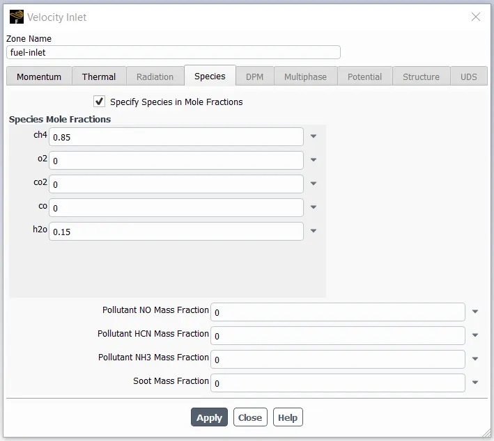
Mole Fraction of `CH_4` `= 0.85` (`85%` fuel)

Mole Fraction of `H_2O` `= 0.15` (`15%` water)

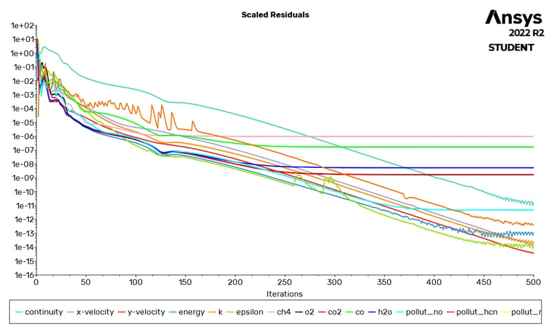
We hybrid initialize the solution and run it for 500 iterations to obtain the following results and plots.

Residuals Plot :

Temperature Plot (Contour & Chart) :

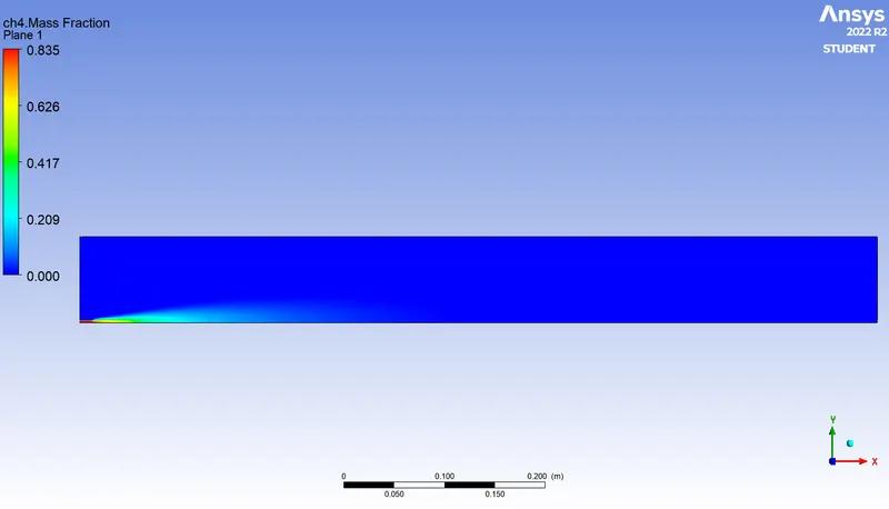
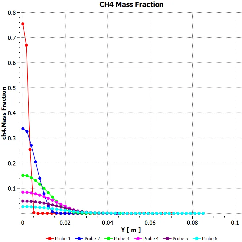
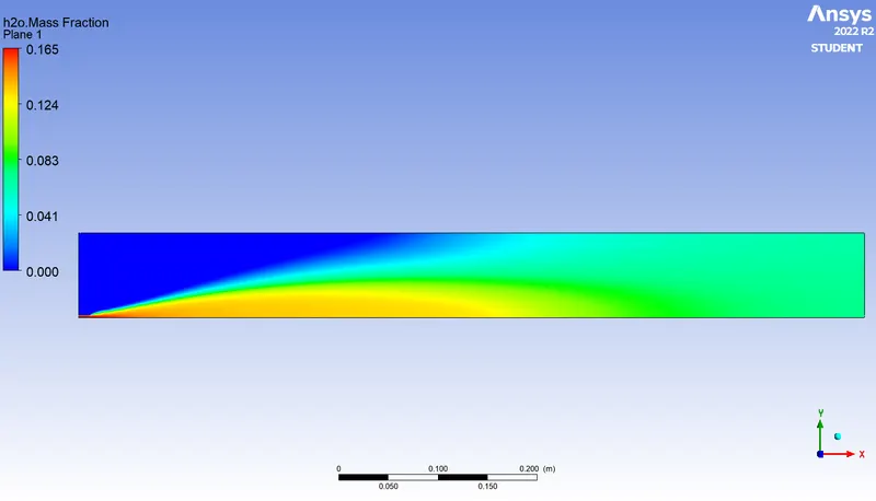
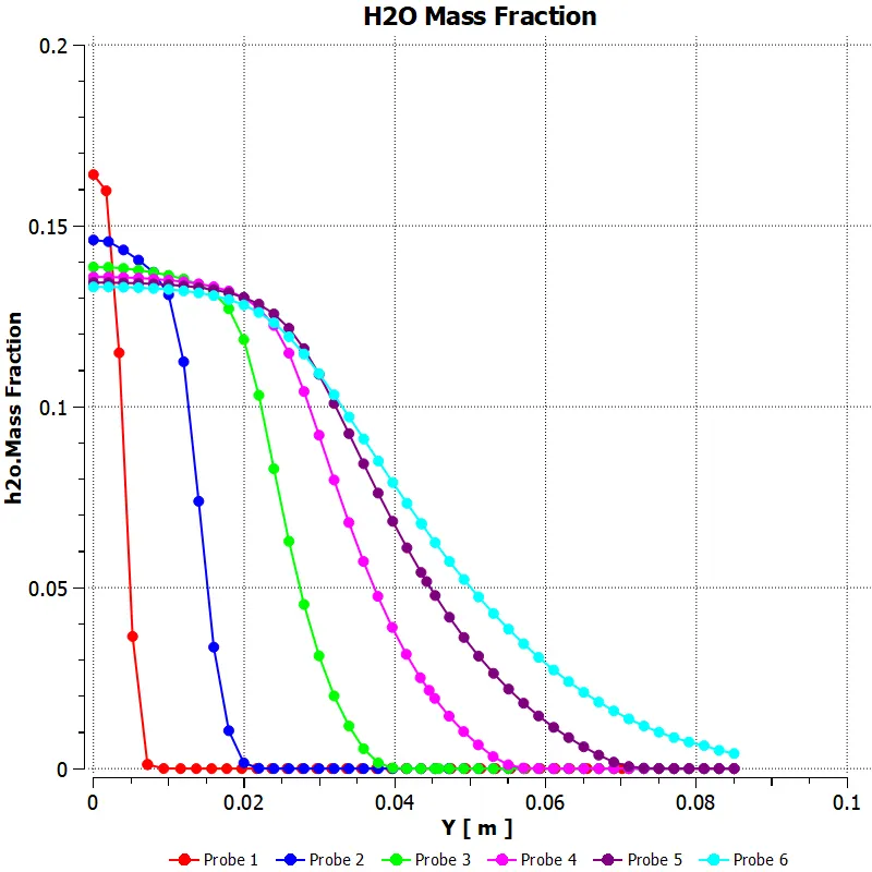
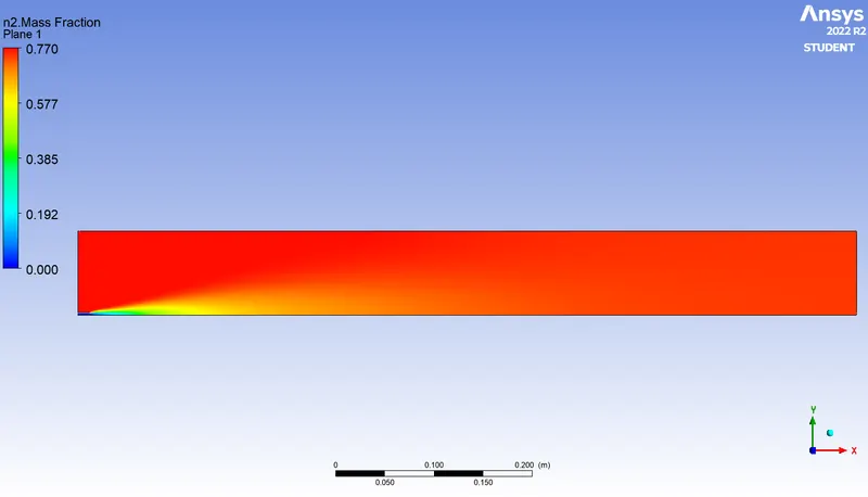
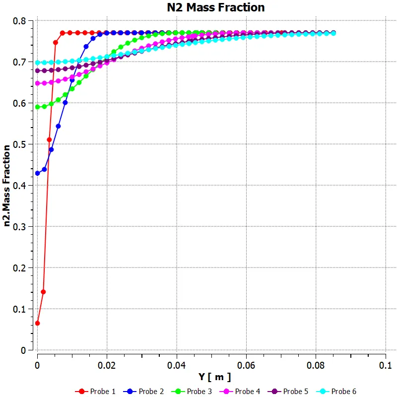
Mass Fractions of Species (Contour & Charts) :

`1.` `CH_4`

`2.` `CO`

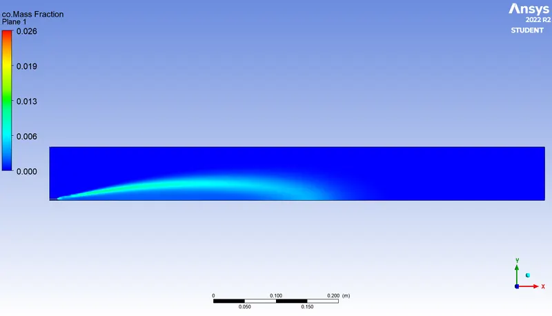
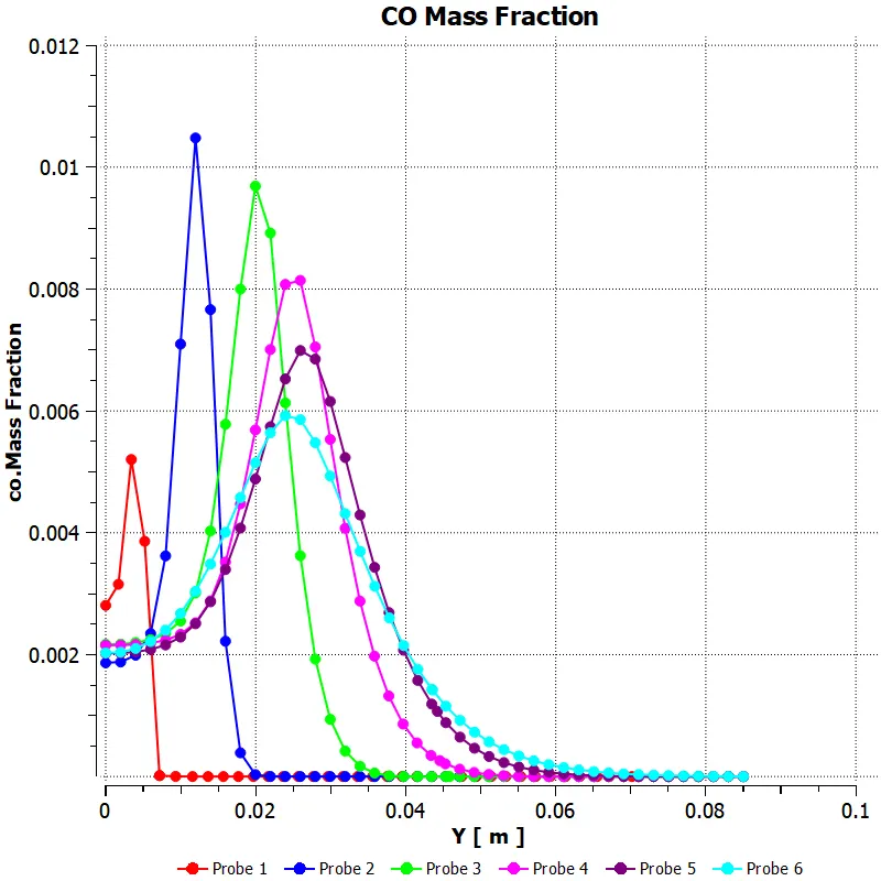
`3.` `CO_2`

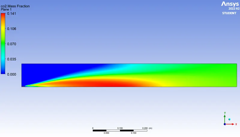
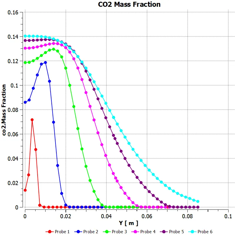
`4.` `H_2O`

`5.` `N_2`

`6.` `O_2`

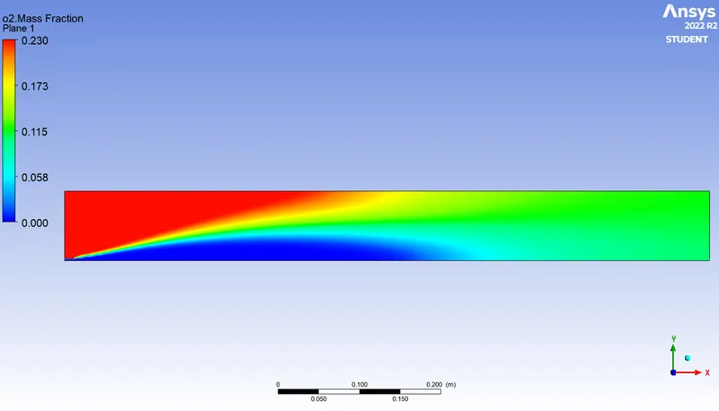
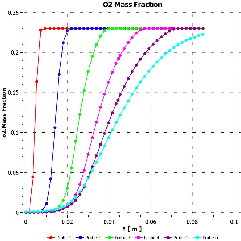
`NO_"x"` Emissions :

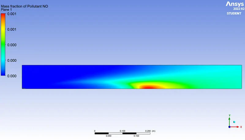
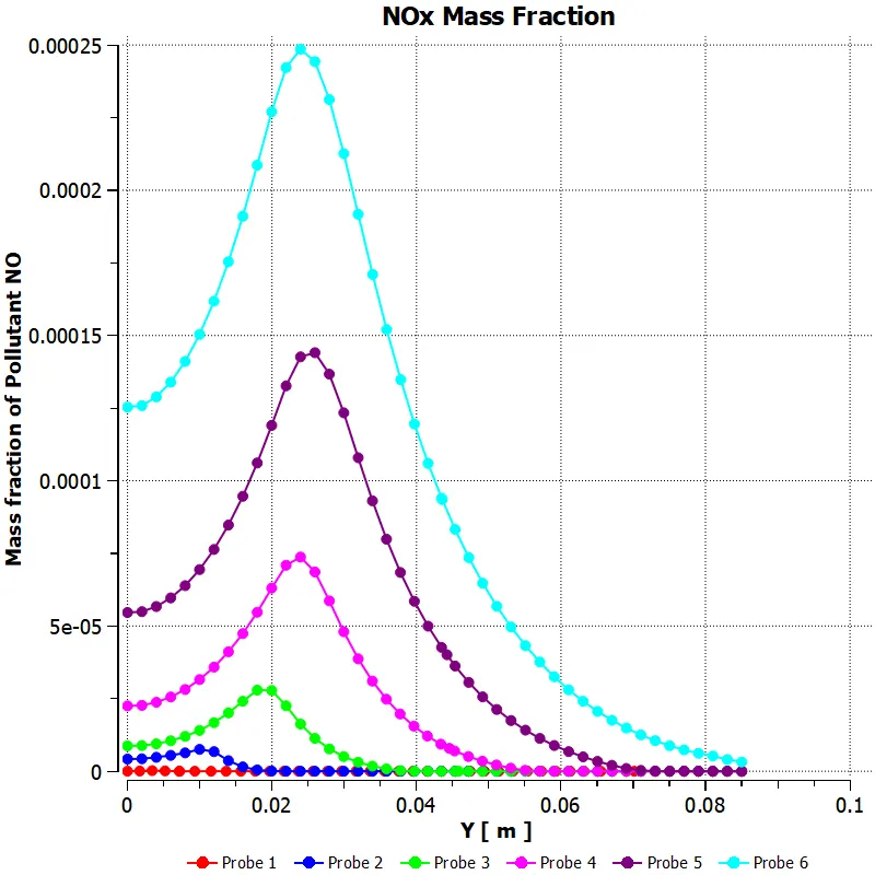
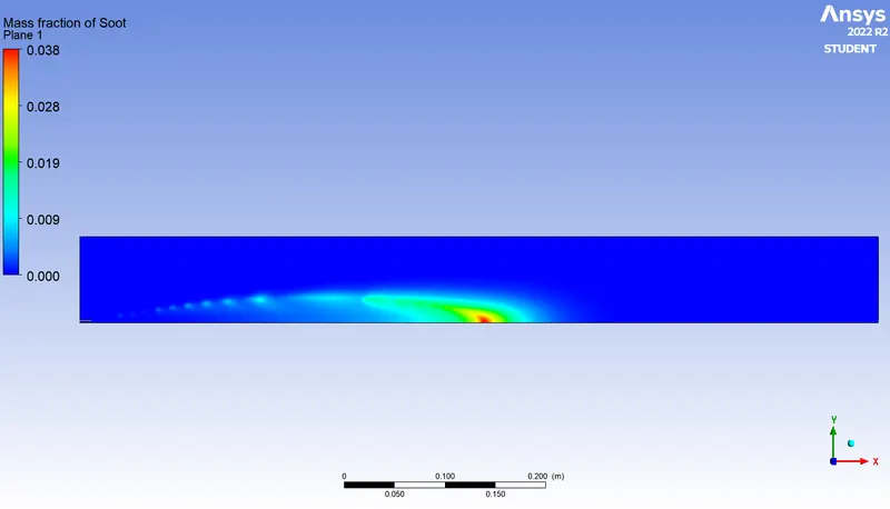
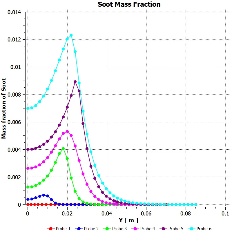
Soot Formation :

CASE – 4 : 30% WATER CONTENT

In this case setup, we increase the water content in the fuel mixture to 30% and we run the simulation to study the effects of this increased water content on the results.

The water content is specified in terms of mole fraction at the fuel inlet as follows.

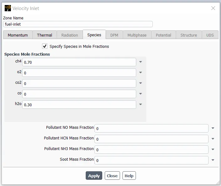
Mole Fraction of `CH_4` `= 0.70` (`70%` fuel)

Mole Fraction of `H_2O` `= 0.30` (`30%` water)

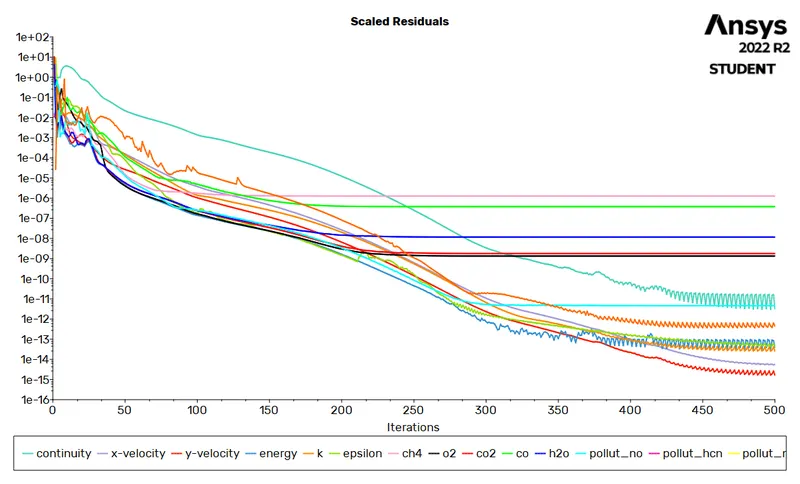
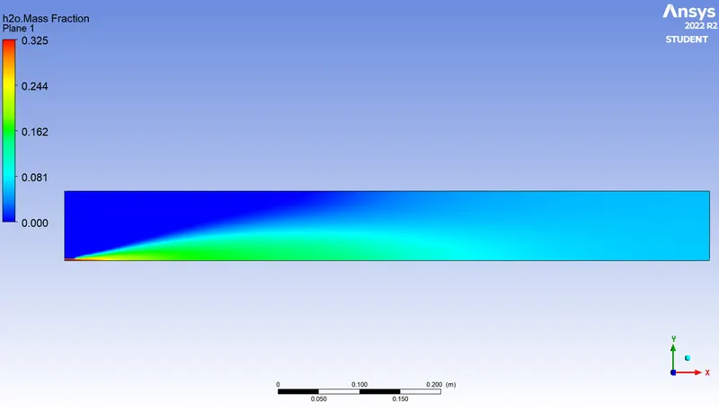
We hybrid initialize the solution and run it for 500 iterations to obtain the following results and plots.

Residuals Plot :

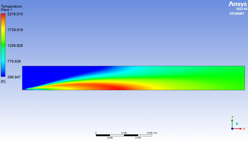
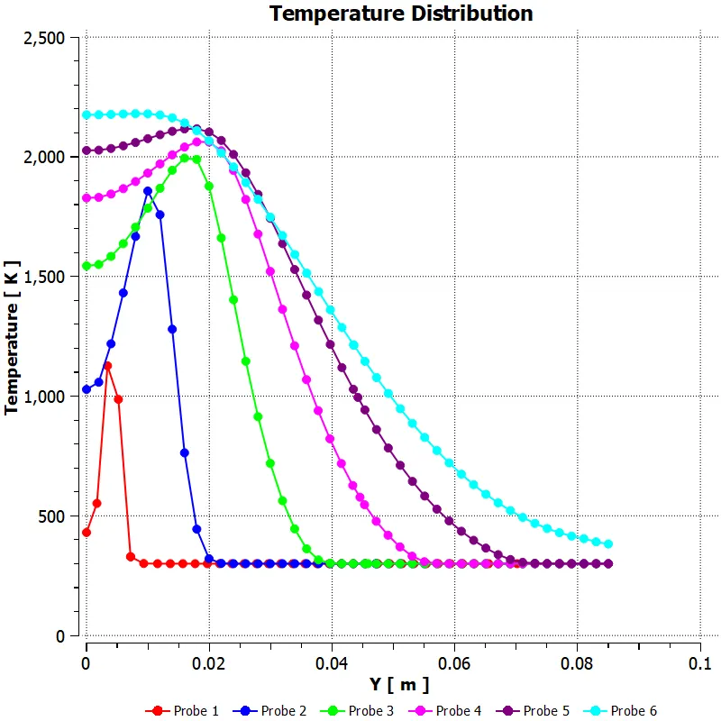
Temperature Plot (Contour & Chart) :

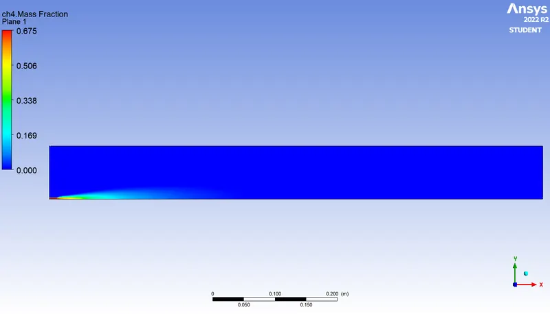
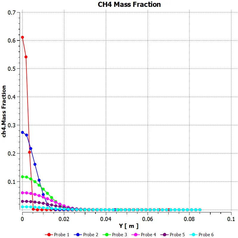
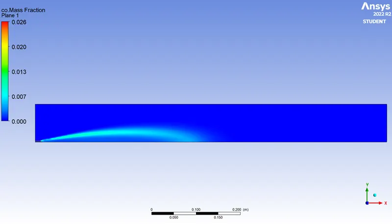
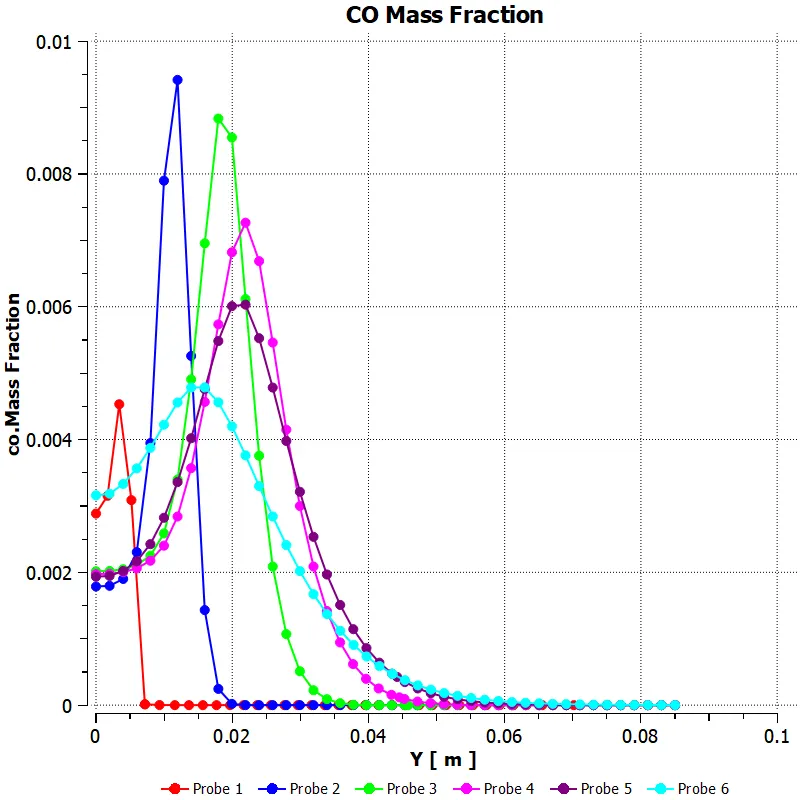
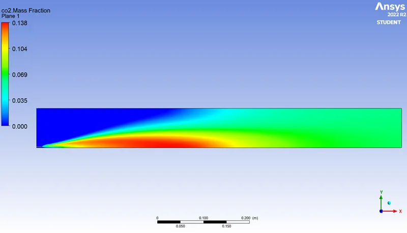
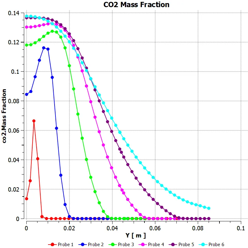
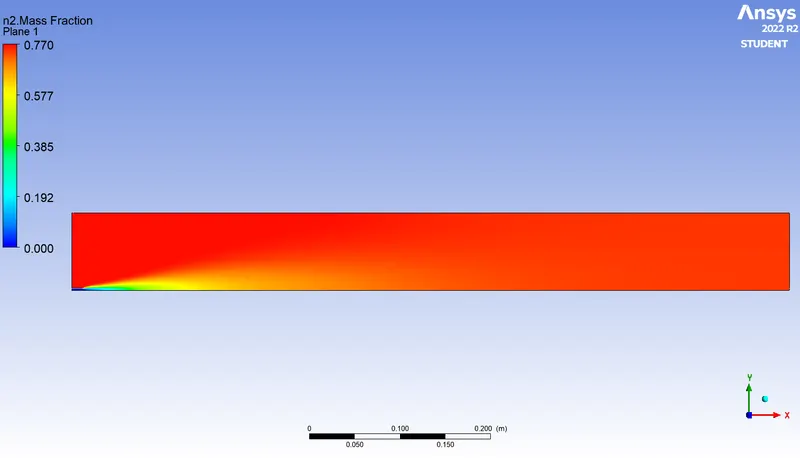
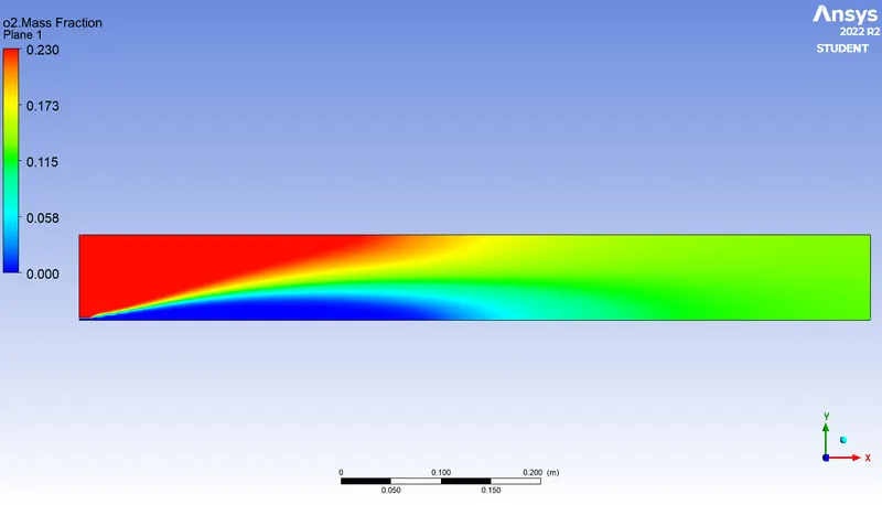
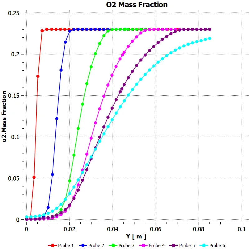
Mass Fractions of Species (Contour & Charts) :

`1.` `CH_4`

`2.` `CO`

`3.` `CO_2`

`4.` `H_2O`

`5.` `N_2`

`6.` `O_2`

`NO_"x"` Emissions :

Soot Formation :

FINAL RESULTS :

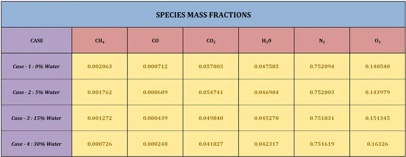
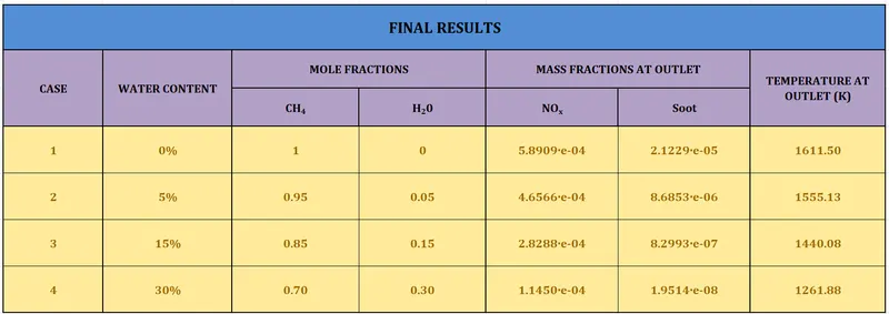
From the above study conducted for various levels of water content in the fuel mixture, we obtain the following values and inferences.

Mass Fractions of the Species :

Case Study Table :

CONCLUSIONS :

The combustion simulation has been successfully carried out for all 4 case studies – representing the different levels of water content present in the fuel mixture (ranging from 0% to 30%). The contour plots as well as the mass fraction graphs, comparing the results at 6 different points (probes) at different regions along the combustor have been obtained.

From the respective mass fraction graphs and values, we can observe that as the water content level in the fuel increases, there is a gradual decrease in the average mass fraction values of CO and CO2. This reduction in the concentration of CO and CO2 gas, leads to the emission products being less harmful to the environment, which is what we are aiming for. Thereby, a higher level of water content in fuel leads to reduction of CO and CO2 mass fractions.

Similarly, we can observe that the mass fractions of N2 almost remain constant even with the variations in water content levels. This thereby affects the flame stability.

From the second table, we can observe that the NOx emissions and Soot formation levels are considerably decreasing with the increase in water content levels. It has been suggested that the added water content reduces the NOX emissions and Soot formation because of the coupling effects of diluting the fuel and oxygen, lowering the flame temperature, and influencing the pathways of chemical reactions in the combustion zone.

Finally, it can be deduced that the increase in water content has a direct effect on the outlet temperature of the combustor. An increase in water content leads to the decrease of the outlet temperature as seen in the case study.