Week 4 - CHT Analysis on Exhaust port

AIM :

To simulate the phenomenon of conjugate heat transfer (CHT) in an exhaust port and carry out its analysis.

OBJECTIVES :

1. Give a brief description of why and where CHT analysis is used.
   
   
2. Calculate the wall/surface heat transfer coefficient on the internal solid surface & show the velocity & temperature contours in appropriate areas.
   
   
3. Verify the HTC predictions from the simulations and explain on what factors the accuracy of the prediction depends on.

INTRODUCTION :

Conjugate heat transfer is a type of heat transfer analysis between solids and fluids. This type of heat transfer includes both convection (between fluids) and conductive (between solids) heat transfer, as well as both forced and natural convection. Common applications and use cases of this thermal simulation type include electronics cooling, heat exchangers, industrial machinery, heaters, some AEC cases, and more.

Heat transfer usually takes place from hotter objects to colder objects. There are three modes of heat transfer.

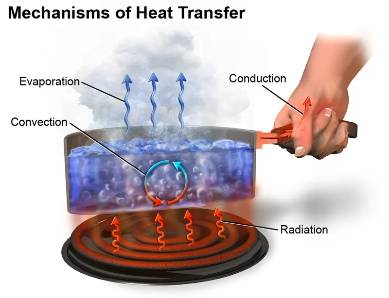
1. Conduction

Conduction is a mode of transmission of heat in which heat is transferred from a region of higher temperature to a region of lower temperature when particles of matter come in direct contact with each other. Particles that have kinetic energy, i.e., motion or heat, can transfer this vibrating motion to another particle that they impact, until the heat is evenly distributed amongst the system of particles.

Examples :

• The heat from a hot liquid making the cup itself hot.
• Ironing a piece of clothing where the heat is transferred to the clothing.
• A heat exchanger using a hot fluid to conduct heat to a cooler fluid, without the two actually coming into direct contact.
• The process of heating a pan on a stove.
• Ice cooling down your hand.

2. Convection

Convection is the transfer of heat related to the movement that occurs within a fluid due to the rising of hotter materials paired with the sinking of colder materials. This occurs because hotter materials have less density than colder ones.

Examples :

• Boiling or water - hot water rises and cooler water moves down to replace it, causing a circular motion.
• Radiator - A radiator puts warm air out at the top and draws in cooler air at the bottom.
• Hot air rising, cooling, and falling (convection currents)

3. Radiation

It is the process in which heat is transferred from one body to another body in the form of electromagnetic waves, without involving the molecules of the medium. Radiation heat transfer does not depend on the medium.

Examples :

• In a microwave, the substances are heated directly without any heating medium.
• Transfer of heat from the sun to earth.

Heat Transfer Co-Efficient :

Heat transfer co-efficient defines the rate of heat transfer between a solid surface and a fluid per unit surface area per unit temperature difference. It refers to how well heat is conducted through a series of resistant mediums.

The general formula of the heat transfer coefficient is:

`h = q / (DeltaT)`

Where,

`q` = Local heat flux density (`W`/ `m^2`)

`h` = Heat transfer coefficient (`W`/`m^2*K`)

`DeltaT` = Temperature difference (`K`)

SIMULATION PROCEDURE :

In this challenge, we are going to carry out a simulation of CHT analysis of an exhaust port. We carry out this procedure through 5 steps by using the Fluid Flow (Fluent) module in ANSYS Workbench. They are as follows.

1. Geometry
2. Meshing
3. Setup
4. Solution
5. Results

1. GEOMETRY

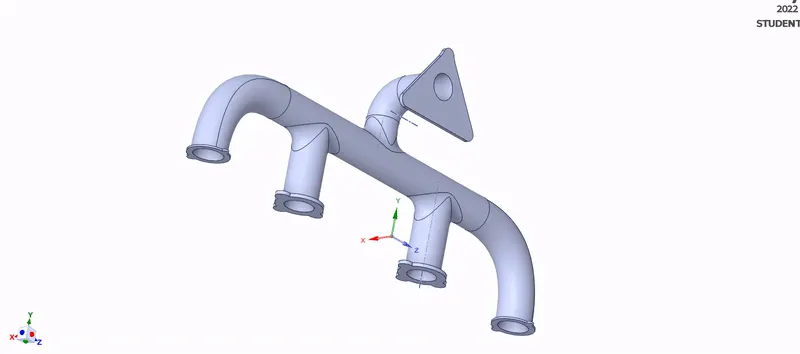
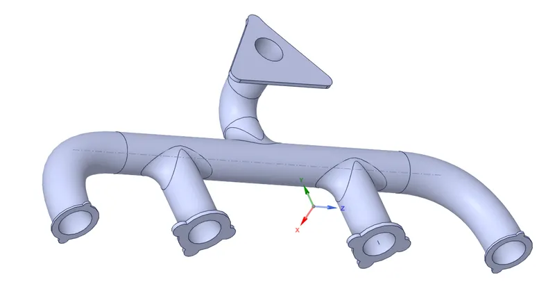
The first and foremost step in the geometry creation is importing the solid model of the geometry into the ANSYS SpaceClaim software. The imported step file is as shown below.

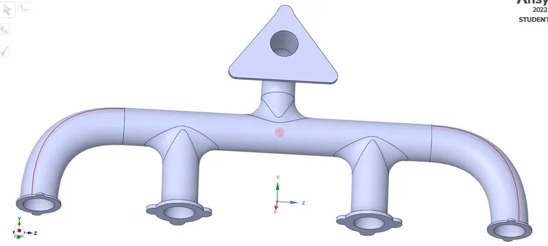
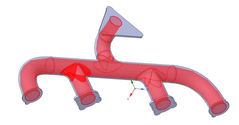
In the next step, we are going to prepare the geometry. To do that, we first repair the geometry by removing the extra edges. The extra edges are as shown in red and thereby, we remove 6 extra edges from the geometry.

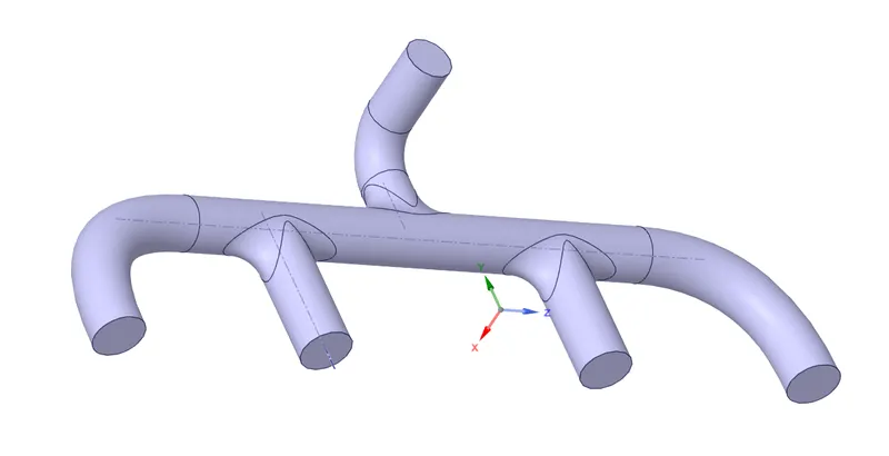
In the next step, we individually extract the solid volume and fluid volume from the geometry by using the volume extract function. Then, we appropriately name it and move it into a separate component representing the final geometries.

Fluid Volume :

Solid Volume :

Finally, we enable share topology, so as to obtain a conformal mesh and also carry out SharePrep function, which thereby shares the co-incident topology. This step takes care of creating interfaces, so that there is just 1 interface between solid and fluid block.

The pink surfaces represent where the information is being shared (co-incident faces).

2. MESHING

After preparing the geometry as shown above, we then move on to the meshing part. The first and foremost step in meshing is to create the named selection faces of the geometry. The inlet, outlet, outer convection wall and the inflation layer faces are named as shown.

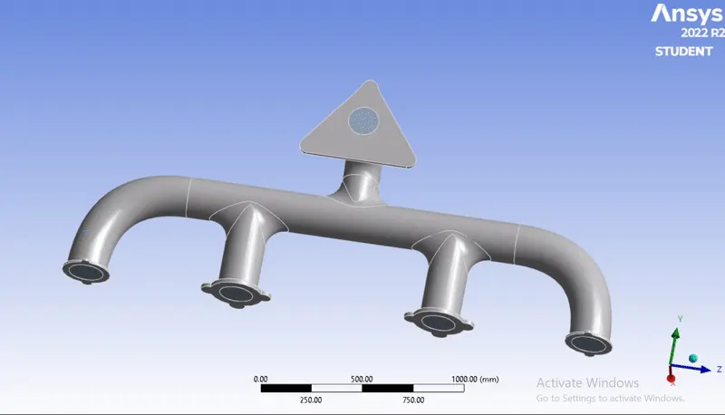
The other additional walls around the inlets and outlet are imported in with adiabatic boundary conditions by default. This means that, these bodies will not allow any heat transfer to take place.

Inflation Layer :

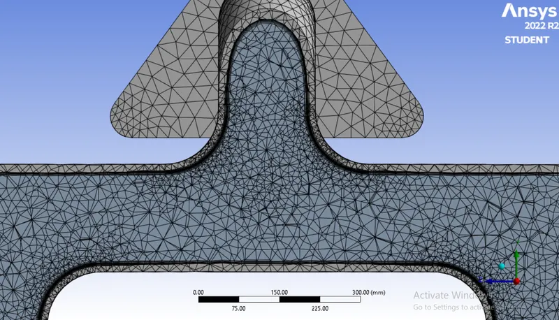
In this step, we create an inflation layer of 5 mm thickness, over and around the co-incident layer, to accurately capture the sharing of information between the solid and fluid surfaces. Inflation layers are created throughout the fluid surface as shown.

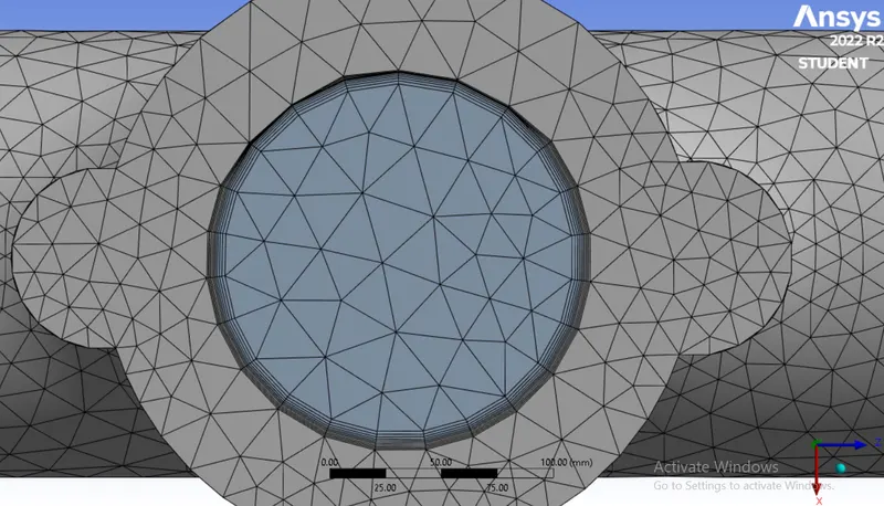
Face Sizing :

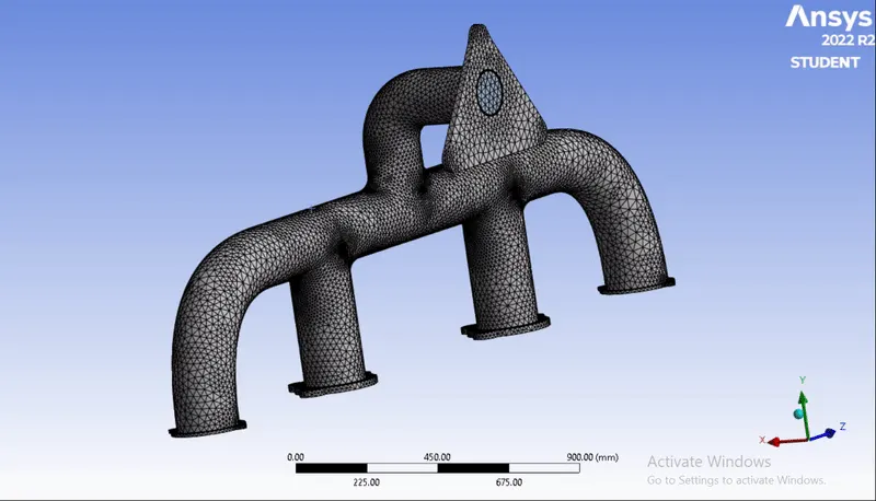
In this step, we create a sizing of 10 mm element size, so as to refine the meshing over the solid and fluid surface. The final meshed model is as shown below.

3. SETUP & SOLUTION

All the surfaces along with the meshing data is imported into the ANSYS Fluent software. The blue surfaces represent the inlets and the red surface represents the outlet of the geometry.

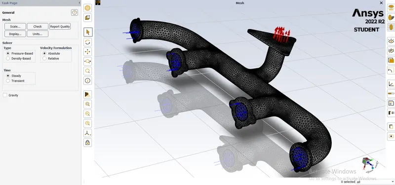
We use a pressure – based solver with absolute velocity formulation and we run the simulation at a steady time state.

Benchmark Parameters :

Solver Type : Pressure – based

Velocity Formulation : Absolute

Time Management : Steady State

Physical Model : Viscous Model

Energy Equation : ON

Turbulence Model : k – omega SST

Fluid Material : Air

Solid Material : Aluminum (al)

Typical Flow Speed : 5 m/s

Inlet Flow Temperature : 700 K

Pressure Outlet : 0 Gauge Pressure (1 atm)

Heat Transfer Co-Efficient : 20 W/m^2.K

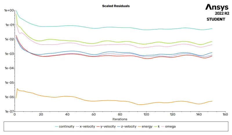
After providing the above mentioned data and conditions, we then initialize (hybrid) the simulation and also define the temperature contours and solution animation to be recorded. Finally, we run the iteration for 150 iterations to obtain the following results.

Residuals Plot :

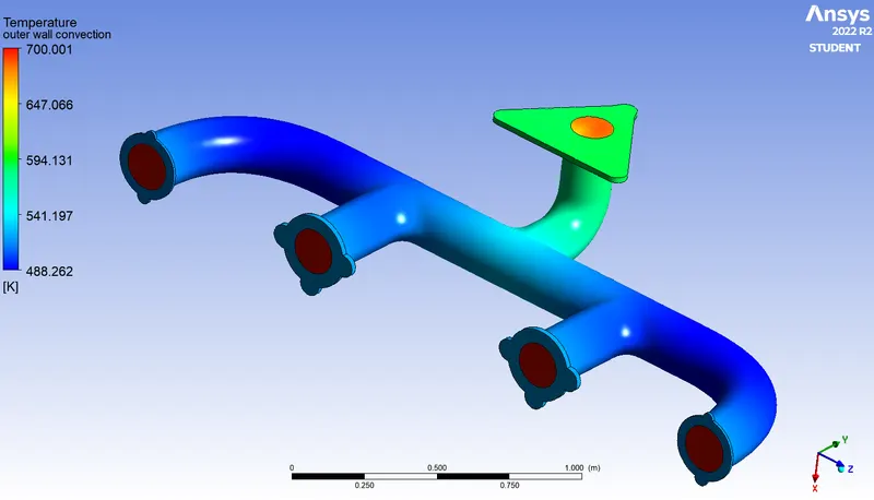
Temperature Contour :

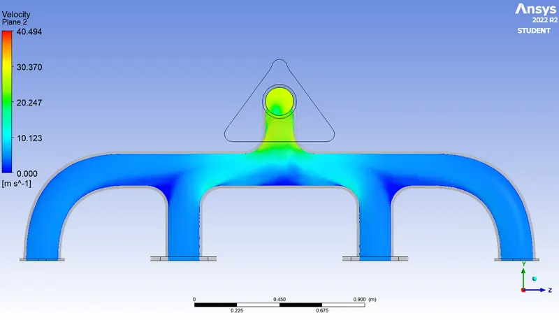
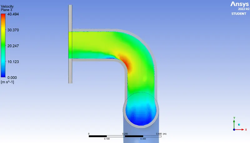
Velocity Contour :

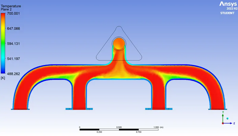
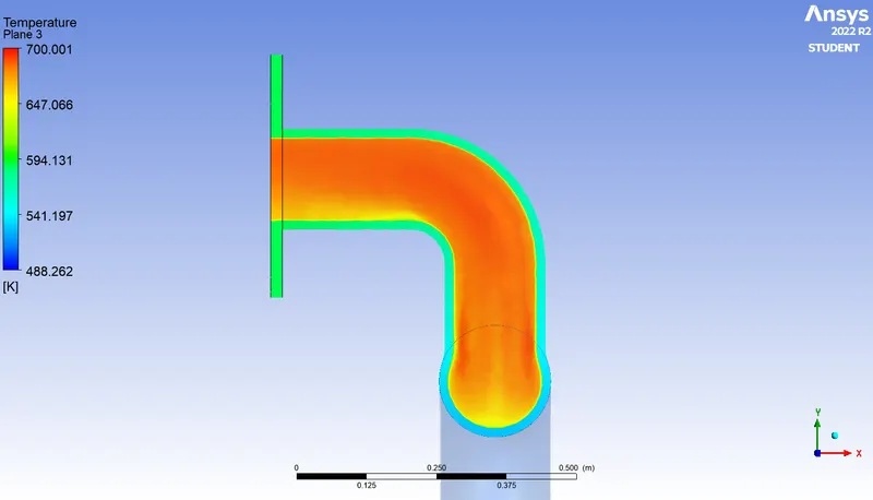
Temperature Plot of Air Flow Through the Exhaust Port :

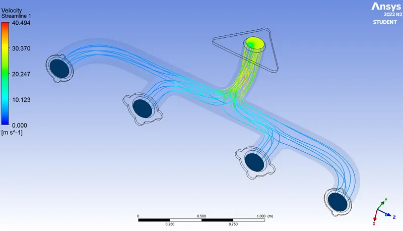
Streamline Velocity Plot :

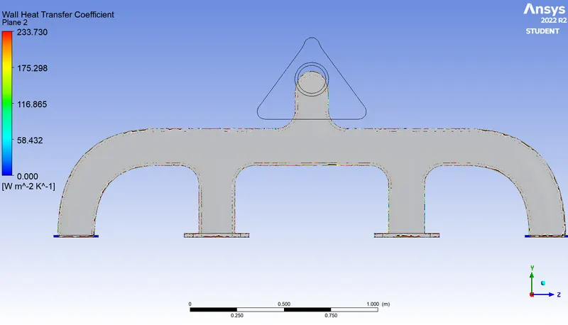
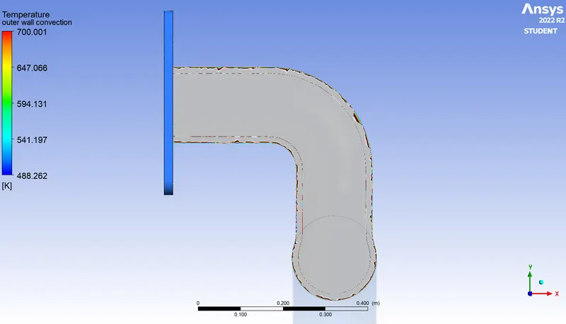
Wall Heat Transfer Co-Efficient :

Verifying HTC Predictions from Simulation :

To verify the HTC predictions, we validate the obtained numerical results with the analytical results by performing calculations using the formulae shown below.

The Reynold’s Number is calculated as,

`Re = (rho * V * D) / mu`

Where,

`rho` = Density of the Fluid (`kg` /`m^3`)

`V` = Fluid Flow Velocity (`m` /`s`)

`D` = Diameter (`m`)

`mu` = Dynamic Viscosity Co-Efficient (`N*s` / `m^2`).

From the obtained Reynold’s Number, we then calculate the Nusselt Number.

`Nu = 0.023 * Re^0.75 * Pr^0.4`

Where,

`Re` = Reynold’s Number

`Pr` = Prandtl Number.

As we know, Nusselt number is the ratio of convective heat transfer to the conductive heat transfer.

`Nu = "Convective Heat Transfer" / "Conductive Heat Transfer"` `= h / (k / L)` `= (hL)/k`

Where,

`h` = Convective Heat Transfer Co-Efficient (`W` / `m^2*K`)

`L` = Characteristic Length (`m`)

`k` = Thermal Conductivity of Fluid (`W`/`m*K`)

From the above relations, we calculate the convective heat transfer co-efficient and we compare it with the numerically obtained values from the simulation and thereby, verifying it.

From the relation, we can say that the flow velocity is directly proportional to the heat transfer co-efficient. This means that, with an increase in velocity of the fluid, the Reynold’s number of the flow is also raised and thereby leading to a higher heat transfer co-efficient value. A high heat transfer co-efficient value means that more heat transfer takes place from fluid to solid surface.

Factors that affect accuracy of the prediction :

1. Accuracy of the geometric model – A precisely modelled geometry gives more accurate results.
2. Wall thickness and other parameters like surface area of the geometry.
3. Share topology – If this is not enabled, then the information between the solid and fluid surfaces are not shared properly.
4. Mesh quality.
5. Inflation layers.
6. Type of solver and turbulence model used.
7. The type of fluid and solid materials used and its properties.
8. Heat transfer co-efficient value.

CONCLUSION :

The conjugate heat transfer analysis of the exhaust port has successfully been carried out and the respective temperature and velocity contour plots have been obtained from the simulation.

From the temperature contour plots, we can observe that the surface temperature of the exhaust port is higher near the outlet, as compared to the inlet, where the hot fluid enters through. We might assume that the surface is going to be the hottest at the inlet but it is infact the opposite. This is because of the phenomenon of convection.

From the velocity contour graphs, we can observe that the fluid velocity is higher near the outlet, as compared to the provided velocity value at the inlet. This is due to the conservation of mass. The air from 4 inlets merge into a single inlet and therefore, the velocity is higher at the outlet.

Finally, we can conclude that the flow velocity is directly proportional to the heat transfer co-efficient. Thereby, higher velocity leads to higher heat transfer co-efficient and hence leading to more heat transfer from fluid to the solid surface.