Week 3 - External flow simulation over an Ahmed body.

AIM :

To simulate the external flow over an Ahmed body.

OBJECTIVES :

1. To run the simulation for a velocity of 25 m/s, with the default air properties in fluent.
   
   
2. Explain the following topics in detail.
   i.) Ahmed's body and its importance.
   ii.) The reason for the negative pressure in the wake region.
   iii.) The significance of the point of separation.
   
   
3. Obtain the velocity and pressure contours along with the drag co-efficient plot for a refined case study.
   
   
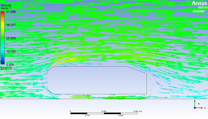
4. Obtain a vector plot clearly showing the wake region.
   
   
   
5. Perform the grid dependence test and provide the values of drag and lift with each case.

INTRODUCTION :

The Ahmed body is a generic car body (a simplified vehicle model). The airflow around the Ahmed body captures the essential flow features around an automobile. Although it has a very simple shape, Ahmed body allows us to capture characteristic features that are relevant to bodies in the automobile industry.

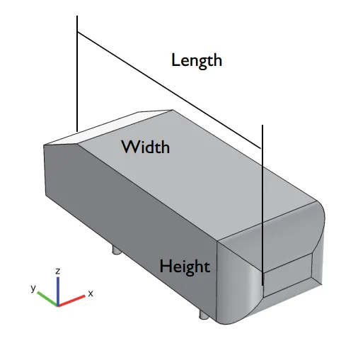
The Ahmed body is designed to have a smooth-edged front end with a flat roof and a flat bottom section and an angled back slant which basically acts as the rear window of a car and ending with a vertical base. The back-slant angle is very critical to the flow patterns which are fashioned at the near wake region and subsequently has an impact on the aerodynamic forces which act on the body.

Importance of Ahmed body :

Ahmed’s body allows us to capture aerodynamic characteristic relevant to bodies in the automobile industry. This model is also used to describe the turbulent flow field around a car-like geometry. When the numerical model is validated, it is used to design new models of the car.

Since the Ahmed body is easy to model, it can be effortlessly utilized for researching various properties like turbulence, drag coefficient, wake region, lift forces, velocity magnitude at various regions of the car, magnitude of pressure around the car which helps in determining what will be resistance, fuel efficiency etc., of the car thereby providing a clear idea on which region needs to be optimized for better effectiveness.

BENCHMARK PARAMETERS :

Typical flow speed = `25` `m`/`s`

Physical model = `"Viscous model"`

Medium = `"Air"`

Reference Density = `1.225` `kg`/`m^3`

Reference Pressure = `1` `"atm"` (`0` `"gauge"`)

Dynamic Viscosity = `1.7894e^-05` `kg`/`m.s`

Turbulence = `"RANS"`

Turbulence Model = `k – omega` `SST` / `"Standard"` `k - epsilon`

Time management = `"Steady State"`

SIMULATION PROCEDURE :

With reference to the above parameters, we are going to carry out our simulation using the ANSYS Workbench software, by the following steps.

MODEL SETUP :

In this step, we import our Ahmed body geometry into the ANSYS SpaceClaim software, where we pre-process it and prepare it for meshing.

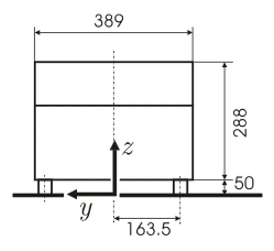
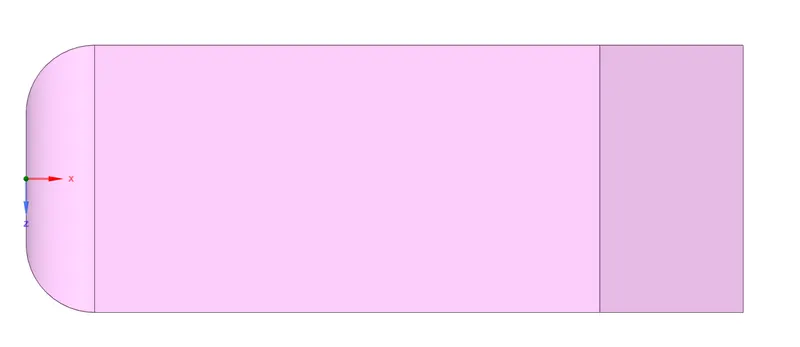
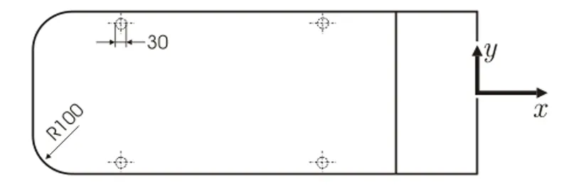
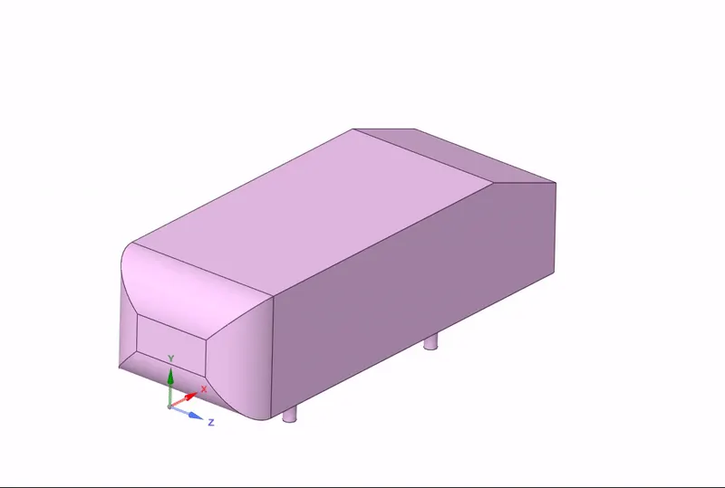
The geometry and views of the Ahmed body is as shown below,

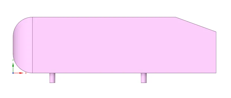
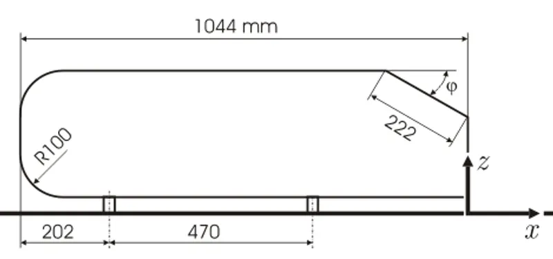
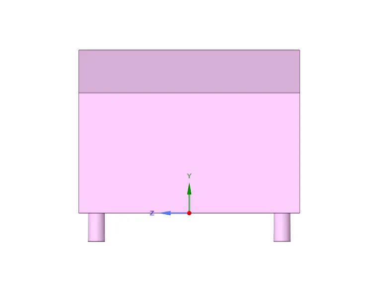
`360^o` Model View :

We are going to carry out the simulation for the above geometry through 3 cases.

1. Base meshing or coarse mesh
2. Medium coarse or partially refined
3. Fine meshing or fully refined.

CASE – 1 : BASE MESHING (1 ENCLOSURE)

In this case study, we are going to simulate the external flow for the Ahmed body with base meshing (default meshing) and study the characteristics.

1. GEOMETRY

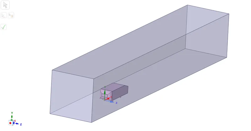
The first step carried out in this simulation is creating an enclosure around the Ahmed body, as we are simulating the flow outside the body. This enclosure is considered to be the domain of the simulation.

We create an enclosure of the following dimensions, as shown below.

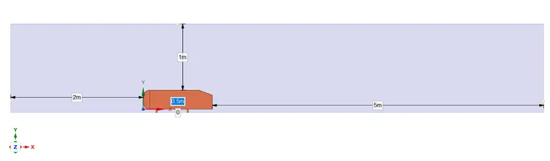
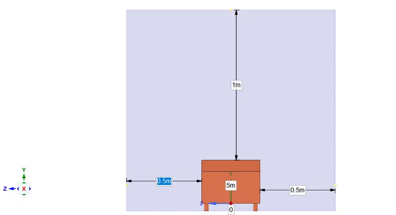
With reference to the above dimensions, we create an enclosure as follows,

Next, we create planes normal to the x, y and z – axes, with respect to the origin. We then create a cut - section, to get a split - view of the geometry.

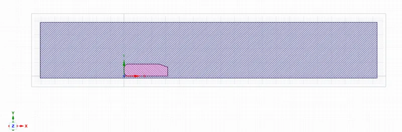
Finally, to make sure that no meshing is generated inside the Ahmed body, we suppress it for physics before moving on to meshing.

2. MESHING

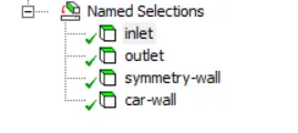
The first and foremost step is creating named selections of the faces namely the inlet, outlet, symmetry walls and the car wall respectively.

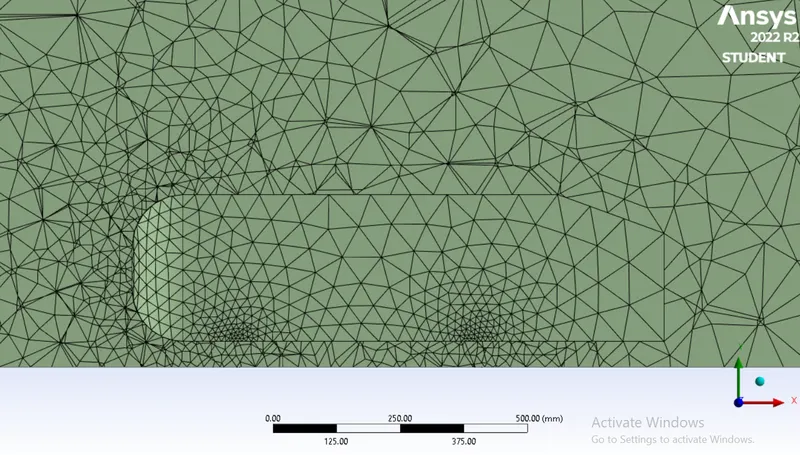
After creating the named selections, we generate the base mesh as shown below.

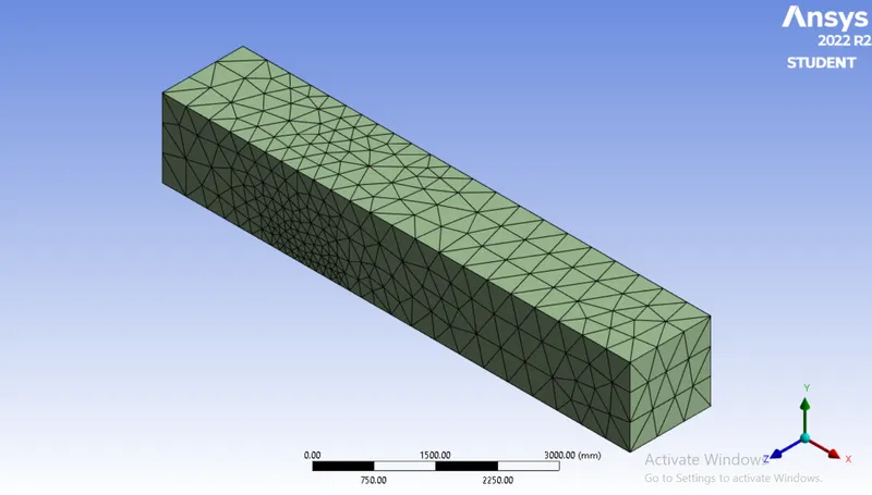
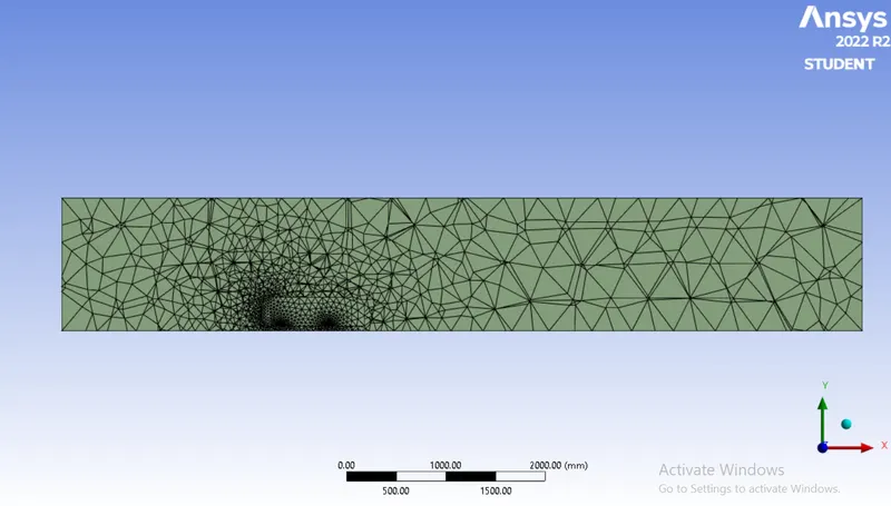
By creating cut – plane, we obtain a sectional - plane view of the mesh.

3. SETUP & SOLUTION :

The first step in the case setup is checking the quality of the mesh using the check mesh utility.

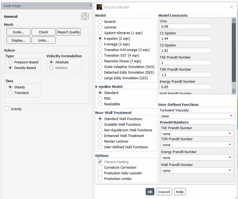
For this case setup, we use a density based solver and a standard k-epsilon turbulence model for simulation. The general setup of the simulation is as shown.

We consider the working fluid to be air at default fluent properties. The following boundary conditions are provided.

• Inlet air velocity is taken as 25 m/s and at an ambient temperature of 300K.
• The outlet is a pressure outlet at 0 gauge pressure (1 atm).
• The car - wall/Ahmed body is provided with a no-slip boundary condition.

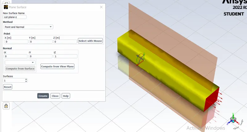
Next, we create a cut plane – z, over which we are going to visualize our velocity and pressure contours.

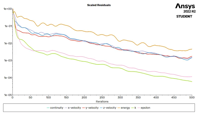
Finally, we initialize (hybrid) the simulation and run it for 500 iterations. We obtain the following results.

Residuals Plot :

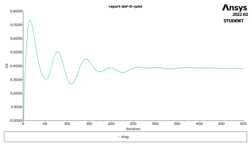
Drag Co-efficient :

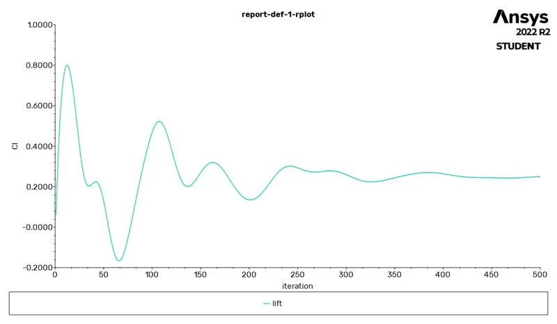
Lift Co-efficient :

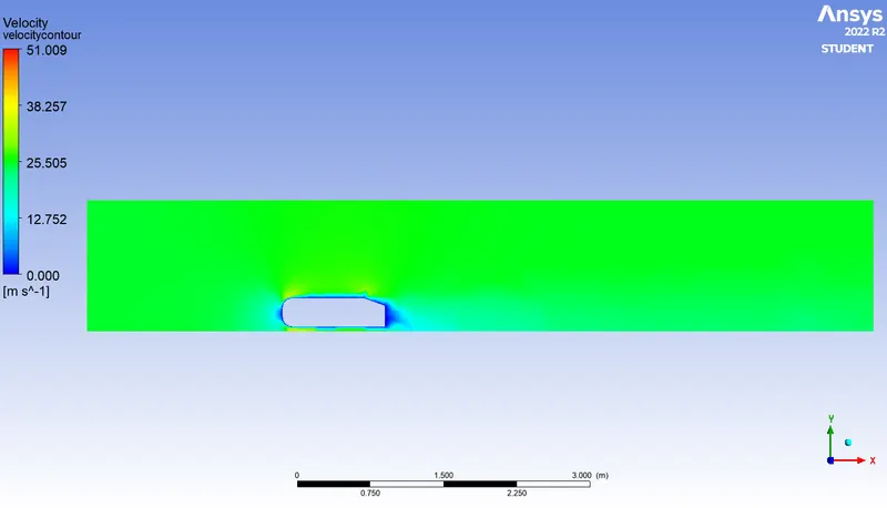
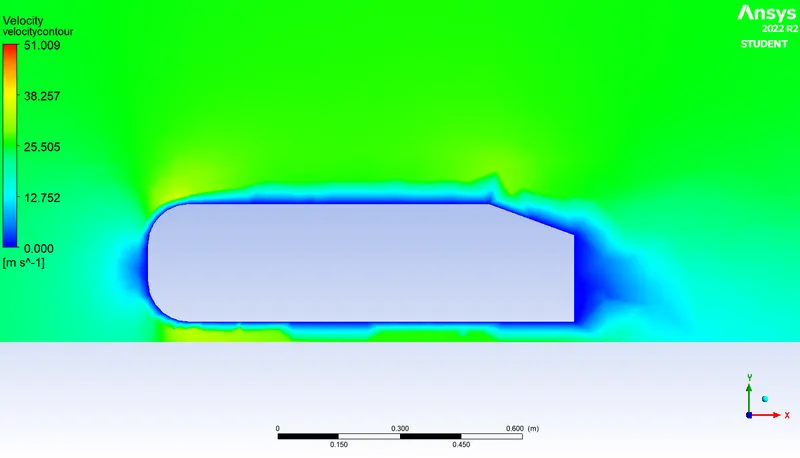
Velocity Contour :

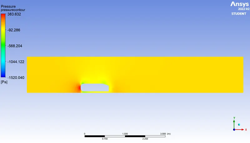
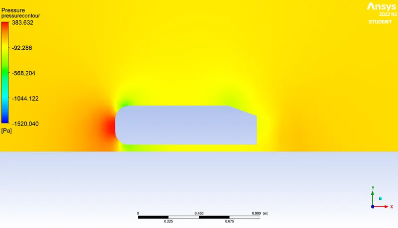
Pressure Contour :

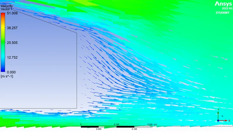
Vector Plot :

Streamline Flow :

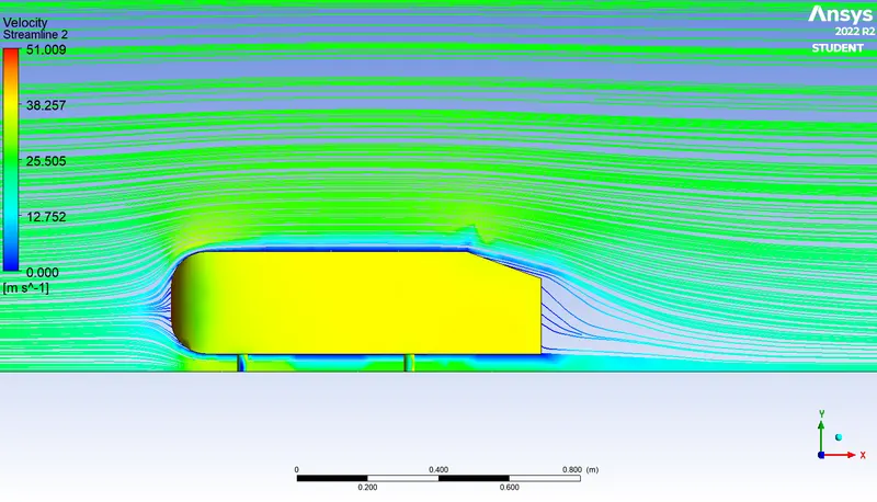
Wake Region :

Output Parameters :

Number of elements = 84064

Drag co-efficient = 0.3826

Life co-efficient = 0.2522

CASE – 2 : MEDIUM COARSE MESH (2 ENCLOSURES)

In this case study, we refine the meshing a bit more, by creating 2 enclosures to accurately capture the fluid flow around the Ahmed body.

1. GEOMETRY

In this step, we create two enclosures around the Ahmed body, inside which it is enclosed. The larger enclosure is considered to be the domain of the simulation and the smaller enclosure is used to create a fine meshing around the Ahmed body so as to capture the flow properties in detail.

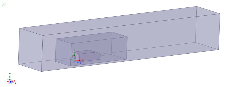
Next, we create a cut-plane so as to obtain a section – view of the geometry. Here, we can observe overlapping of the bodies or enclosures. Therefore, we use the interference function to detect and fix the interfering bodies as shown below.

Before :

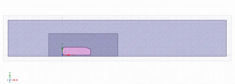
Interference Function :

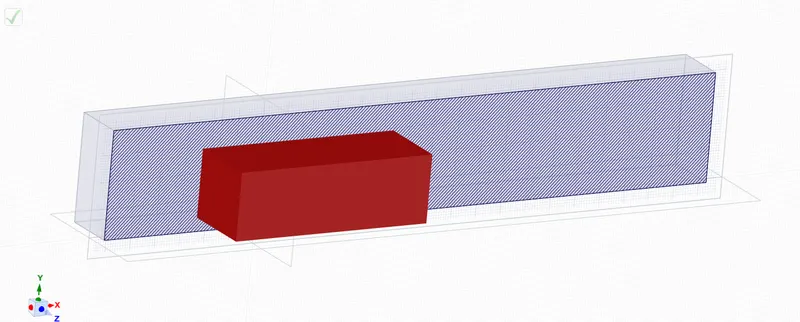
After :

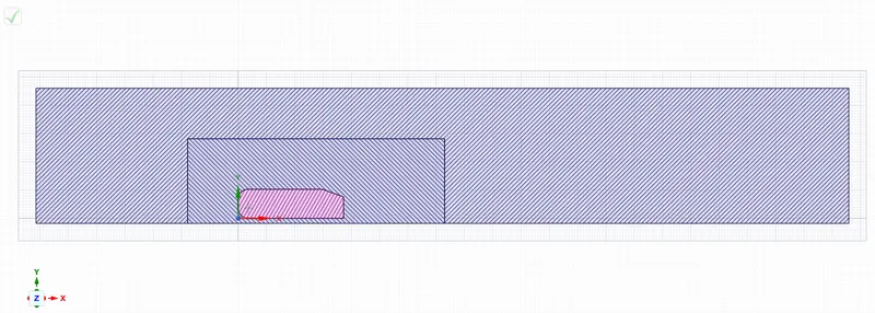
Thereby, the interference has been resolved and we can move onto meshing.

2. MESHING

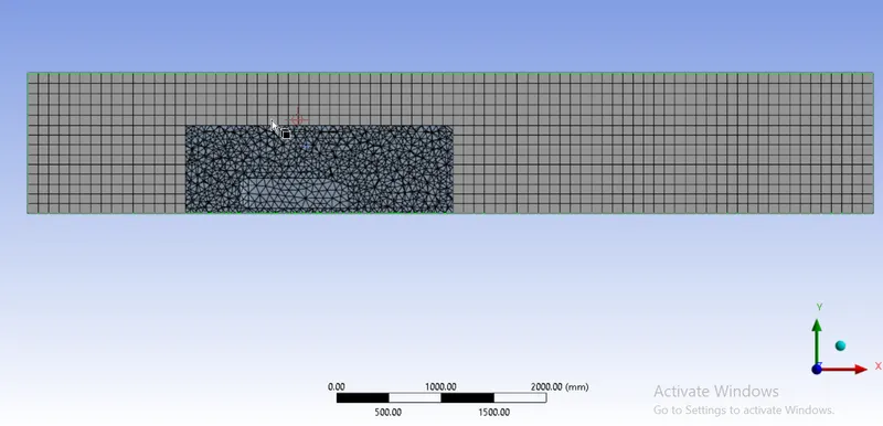
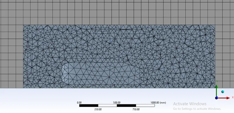
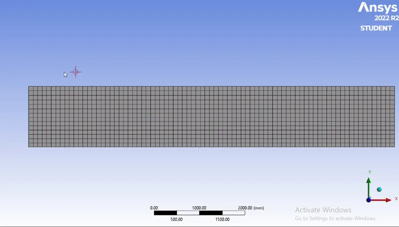
In this process, we create hexahedral meshing in the domain region. To do that, we use multizone meshing, which creates hexahedral meshing wherever possible and in other regions, a different kind of mesh is generated.

For this case study, we use a meshing element size of 100 mm for the bigger enclosure and an element size of 75 mm for the smaller enclosure. The meshing is obtained as shown below.

`360^o` view of Meshed Model :

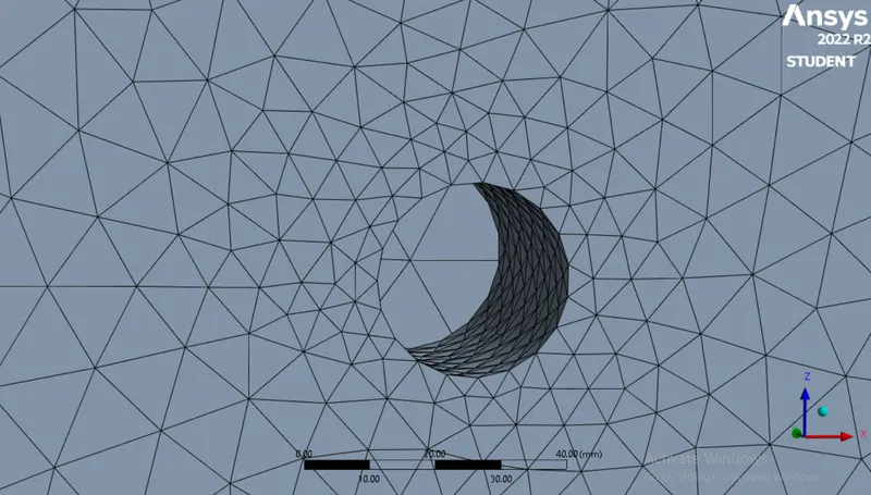
If we zoom into the 4 holes (legs) of the geometry, we can observe that it has been approximated as polygons. Hence, we refine these holes by face sizing. We refine it to an element size of 5 mm.

Before :

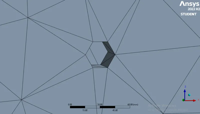
After Face Sizing :

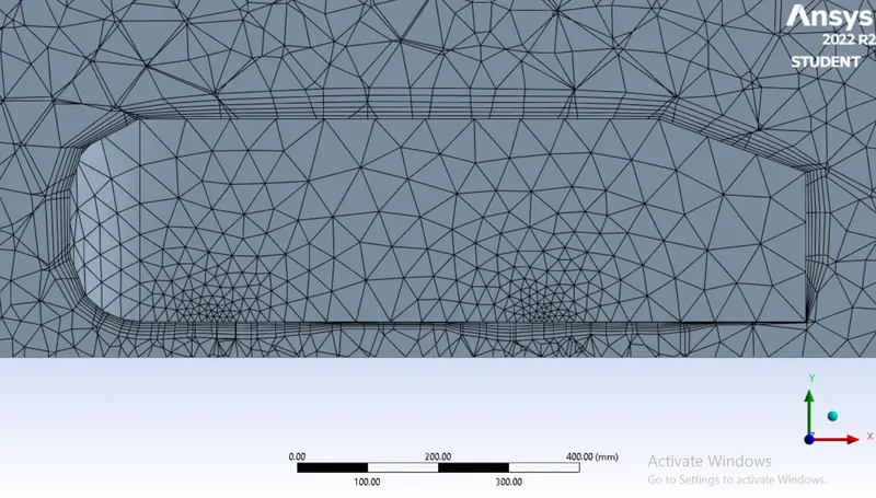
Finally, we create a body fitted inflation layer around the Ahmed body, so as to accurately capture the flow characteristics of the fluid around the Ahmed body. We create 6 inflation layers with the first layer thickness being 5 mm and a growth factor of 1.2.

3. SETUP & SOLUTION

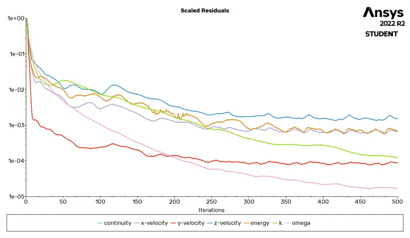
For this case setup, we use a density based solver and a k-omega SST turbulence model for simulation. The general setup of the simulation is as shown.

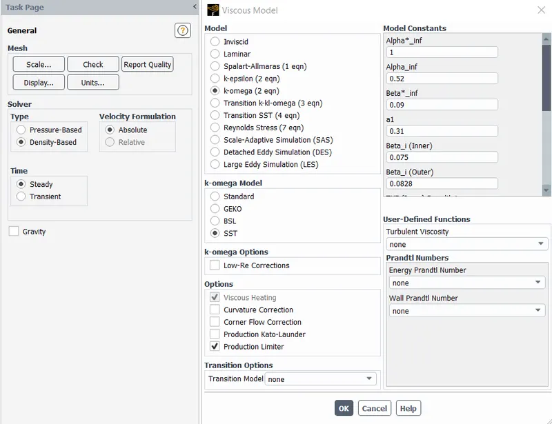
We then provide the respective boundary conditions, initialize (hybrid) the simulation and run it for 500 iterations to obtain the following results.

Residuals Plot :

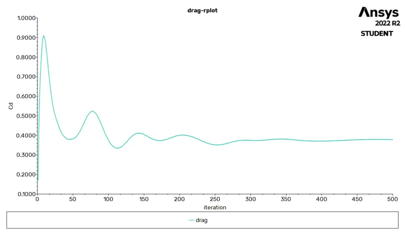
Drag Co-efficient :

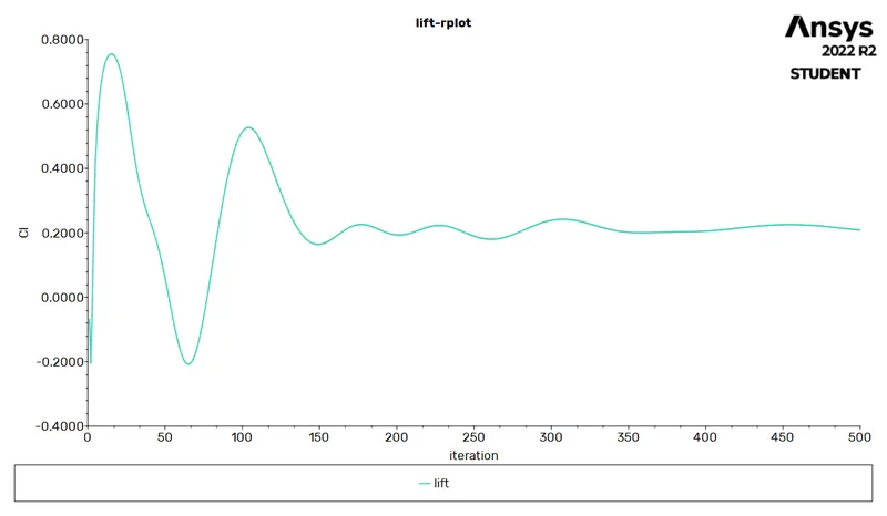
Lift Co-efficient :

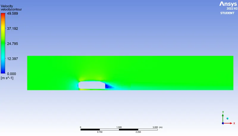
Velocity Contour :

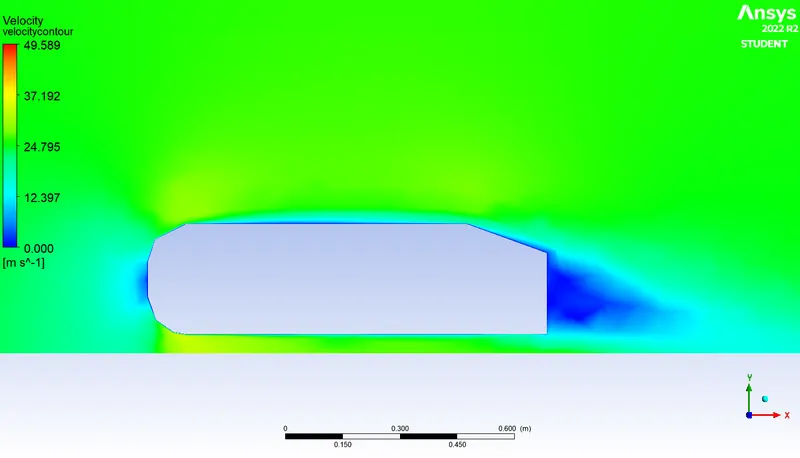
Pressure Contour :

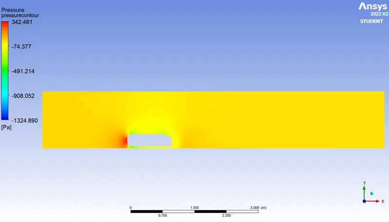
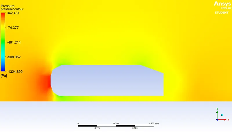
Vector Plot :

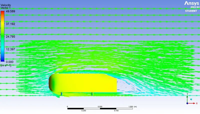
Streamline Flow :

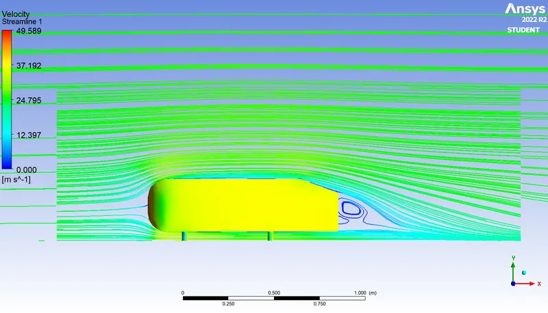
Wake Region :

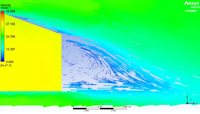
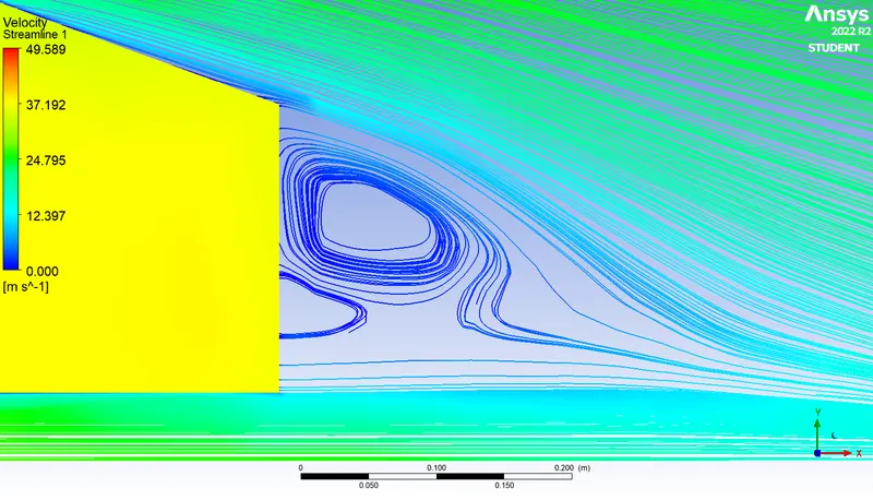
Output Parameters :

Number of elements = 102652

Drag co-efficient = 0.3772

Life co-efficient = 0.2065

CASE – 3 : REFINED MESH

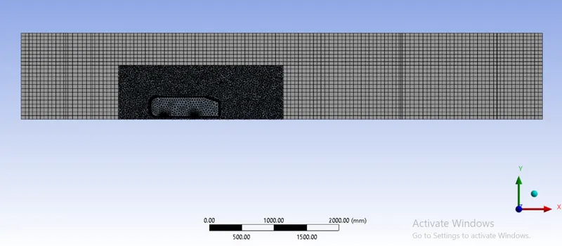
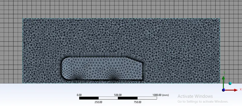
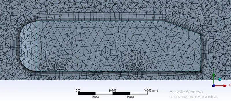
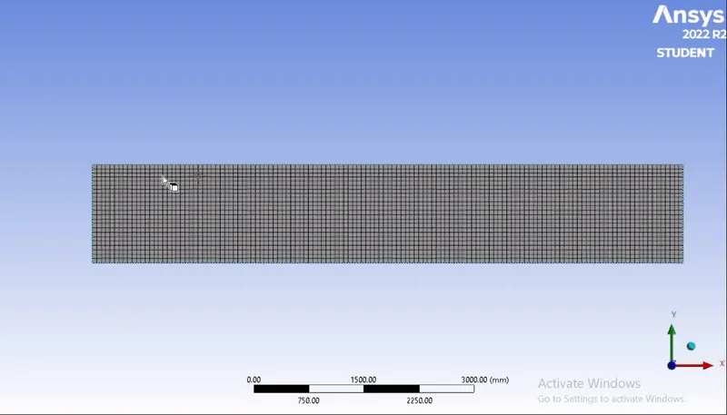
In this case study, we refine the mesh by using an element size of 60 mm for the bigger enclosure (hexahedral meshing) and an element size of 35 mm for the smaller enclosure. Also, we create 10 inflation layers with the first layer thickness being 2 mm and a growth factor or 1.2, so as to capture the flow properties around the Ahmed body more accurately.

Meshing :

Inflation Layer :

`360^o` view of mesh model :

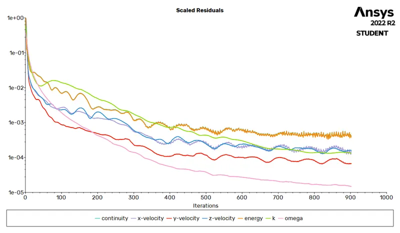
For the simulation, we use a density based solver and a k-omega SST turbulence model. We run the simulation for 900 iterations to obtain the following results.

Residuals Plot :

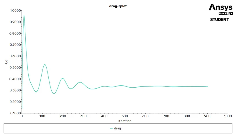
Drag Co-efficient :

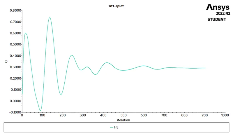
Lift Co-efficient :

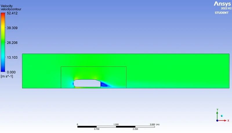
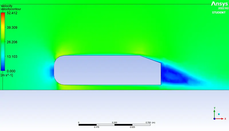
Velocity Contour :

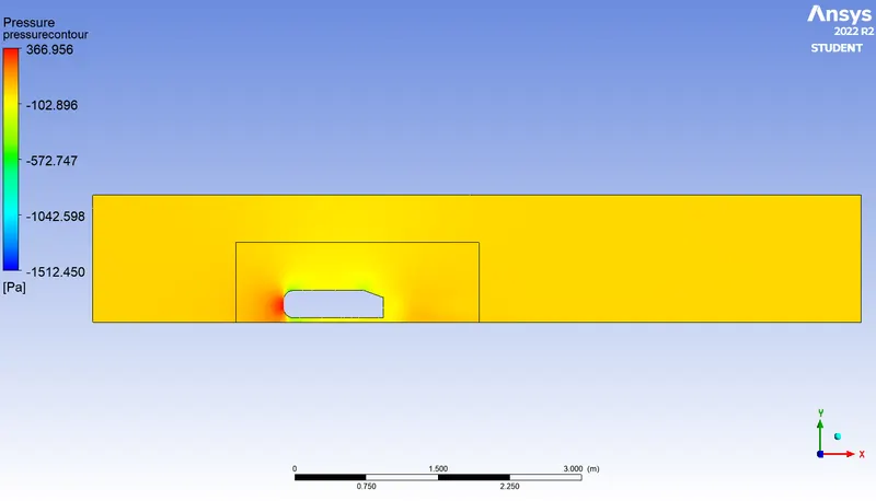
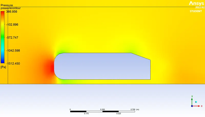
Pressure Contour :

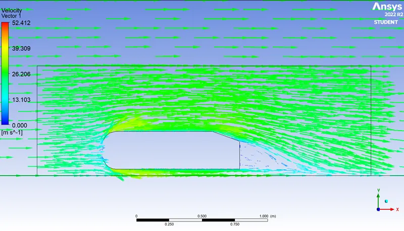
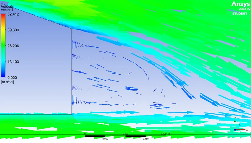
Vector Plot :

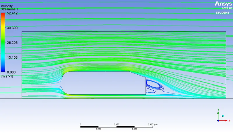
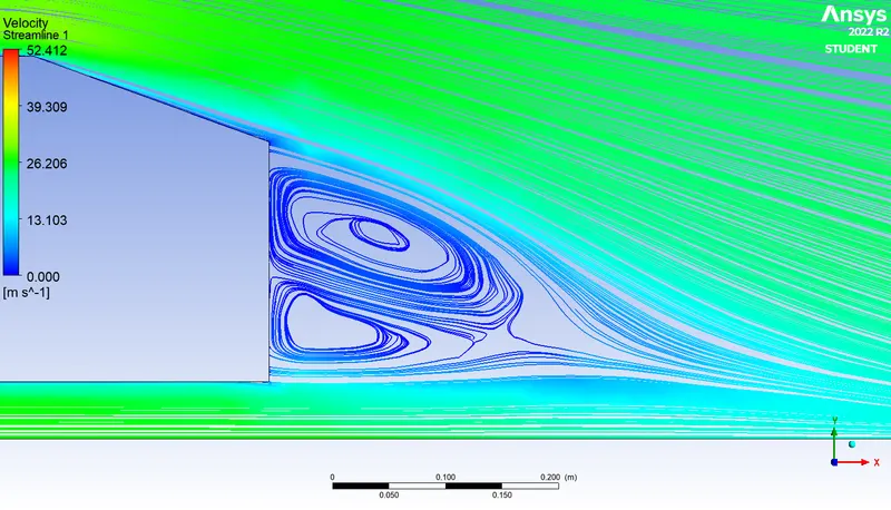
Streamline Flow :

Wake Region :

Output Parameters :

Number of elements = 493966

Drag co-efficient = 0.3315

Life co-efficient = 0.2897

Q1. Explain the reason for the negative pressure in the wake region.

The flow behind an object separates from the surface and creates a highly turbulent region behind the object, called the wake. The pressure inside the wake region remains low as the flow separates and a net pressure force (pressure drag) is produced. This difference in pressure increases the drag due to the pressure drop behind the Ahmed body

In other words, due to the production of pressure drag from flow separation, the pressure in the wake region is low. This is what is causing the vacuum.

Q2. Explain the significance of the point of separation.

In fluid dynamics, flow separation or boundary layer separation is the detachment of a boundary layer from a surface into a wake.

Flowing against an increasing pressure is known as flowing in an adverse pressure gradient. The boundary layer separates when it has travelled far enough in an adverse pressure gradient that the speed of the boundary layer relative to the surface has stopped and reversed direction. The flow becomes detached from the surface, and instead takes the forms of eddies and vortices. The fluid exerts a constant pressure on the surface once it has separated instead of a continually increasing pressure if still attached.

In aerodynamics, flow separation results in reduced lift and increased pressure drag, caused by the pressure differential between the front and rear surfaces of the object.

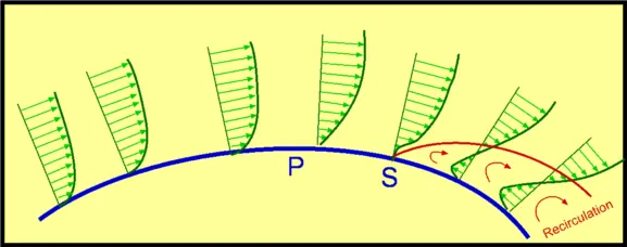
Consider flow past a curved surface as shown above. The geometry of the surface is such that we have a favourable gradient in pressure to start with and up to a point P. The negative pressure gradient will counteract the retarding effect of the shear stress (which is due to viscosity) in the boundary layer. For the geometry considered we have an adverse pressure gradient downstream of P.

FINAL RESULTS :

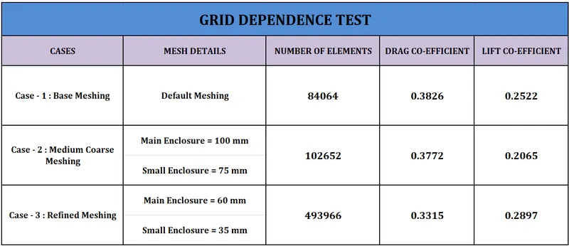
By running the simulation for the 3 case studies as mentioned above, we obtain the following results.

CONCLUSIONS :

The grid dependency test allows us to see smoother velocity profile. As we make the mesh finer i.e. when we increase the cell counts (closer to the limit), we can see from the vector plots from all the 3 cases, of the velocity that it becomes more and more smoother. One thing is observable that making the mesh finer lets us see the wake region more prominently. From the 3 cases, we can conclude that the flow is more defined at lower element size i.e. at case 3. The finer the mesh gets, the easier it gets in visualizing the contours. Mesh refinement increases the closeness of the resulting values to the true values.

Local refinement of the enclosure is a great tool for performing analysis and it improved the results without which wouldn’t have been so accurate. This study for all practical purposes gives a great real-world scenario of aerodynamic impact on a car body, which when improved can help overcome many challenges faced by automobiles.