Week 2 Challenge : Surface meshing on a Pressure valve
AIM :
To generate surface meshing for the pressure valve geometry for 3 different target lengths.
OBJECTIVES :
1. To check for the geometrical errors and perform Topology clean-up accordingly, for the given model.
2. Set three different target lengths as three different cases and mesh the model.
- Target length = 1mm, 3 mm and 5 mm (i.e., 3 cases)
- Element type = Tria.
3. Write a detailed report on the meshing process and explain which case is giving good results and why.
INTRODUCTION :
A relief valve or pressure relief valve (PRV) is a type of safety valve used to control or limit the pressure in a system. Pressure might otherwise build up and create a process upset, instrument or equipment failure, or fire. The pressure is relieved by allowing the pressurized fluid to flow from an auxiliary passage out of the system.
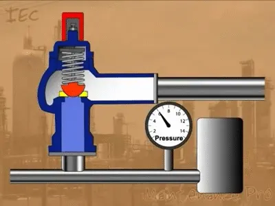
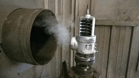
When the set pressure is exceeded, the relief valve becomes the "path of least resistance" as the valve is forced open and a portion of the fluid is diverted through the auxiliary route. As the fluid is diverted, the pressure inside the vessel will stop rising. Once it reaches the valve's reseating pressure, the valve will close.
PROCEDURE :
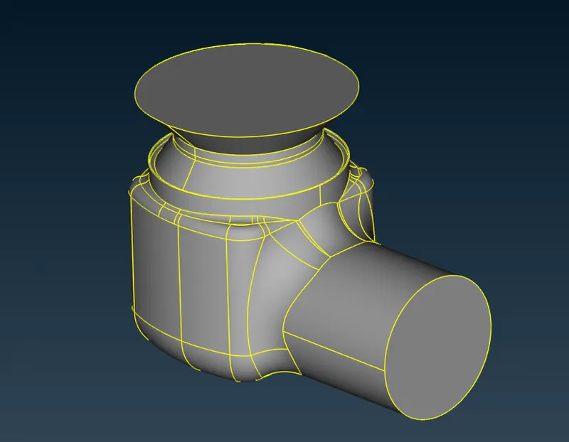
The first and foremost step to be carried out is importing the given geometry model into the ANSA software. The imported geometry of the pressure valve is as shown.
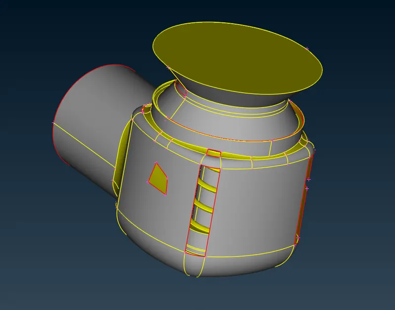
As we can observe, the imported geometry contains various missing surfaces, single CONS and various other such errors. We first need to resolve all these errors before meshing the geometry. We do this in various steps, namely.
1. TOPO CLEAN-UP
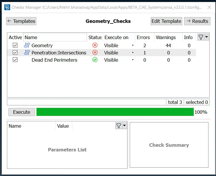
In this step, we first run a geometry check by using the check manager, so as to figure out all the errors and warnings in the geometry. We can see that it displays various errors such as geometry and intersection errors, which we need to resolve one by one.
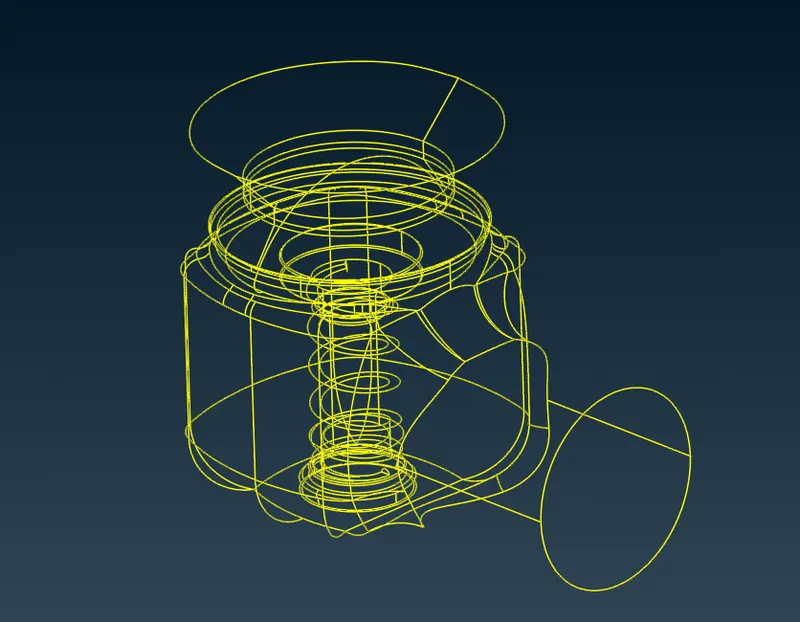
These errors can also be visualized in the wireframe mode as shown.
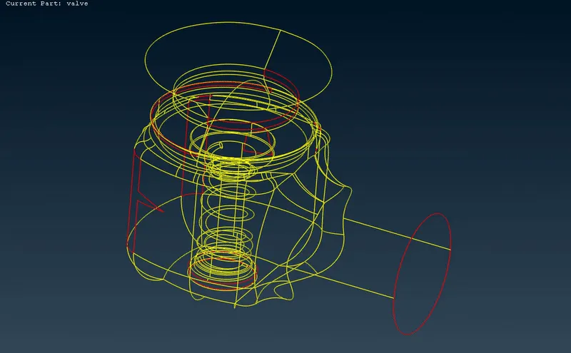
We now resolve these errors one by one. The first step is resolving the surface errors such as the missing faces, small holes and so on. We do this by creating a new COONS face enclosed by the single CONS, as well as by using the “fill hole” function, so as to cover up all the open surfaces and thereby getting rid of all the single CONS in the process. We create new surfaces as shown.
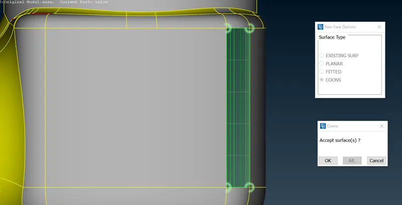
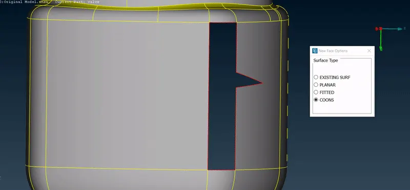
For this surface, we use a combination of creating a new face and the fill hole function to cover the surface as follows.
We use the planar face option to cover the outlet region of the pressure valve.
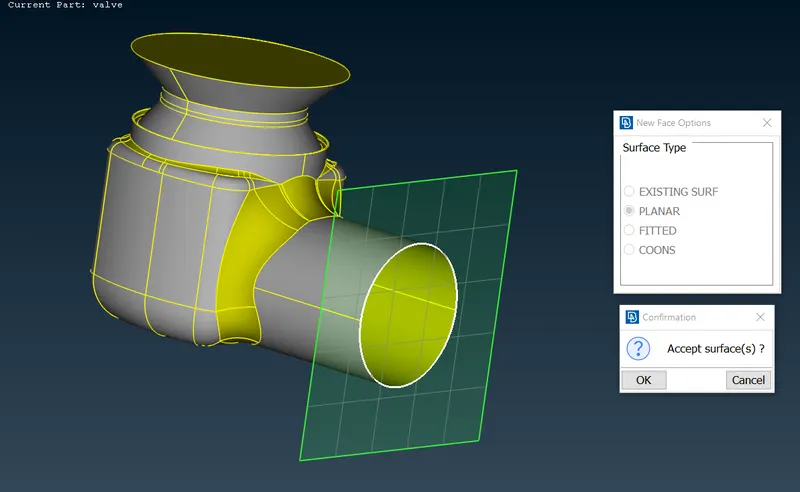
Finally, we orient the geometry to display grey surfaces on the outside and yellow surface on the inside. Thereby, we solve all the surface errors of the geometry by creating new faces. We can observe that there are no more double CONS left and hence, the geometry errors have been resolved.
2. PID CREATION
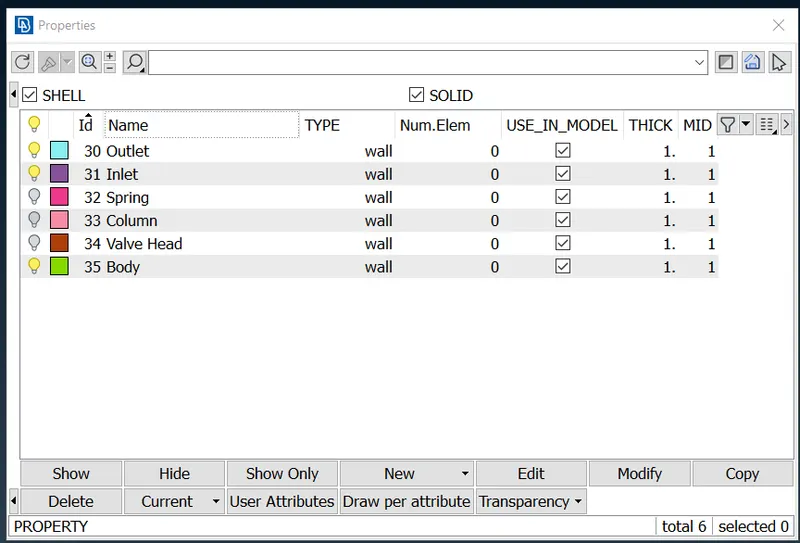
After the topo clean-up of the geometry, the next step is assigning the property ID’s (PID’s) to the various components of the pressure valve. Each component is visualized by a different colour, representing its particular PID.
The various components of the valve are marked as follows.
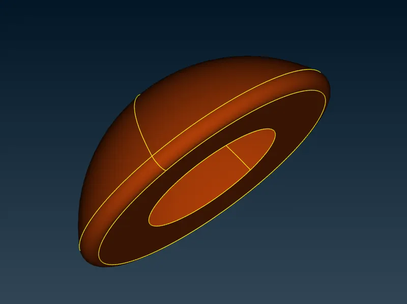
i.) Valve Head
The valve head is configured to make a seal on a valve seat. In operation, when the force of the upstream pressure exerts a greater force than the spring force, then the valve head moves away from the valve seat which allows fluid to pass through to the outlet port. As the upstream pressure drops below the set point, the valve head then closes.
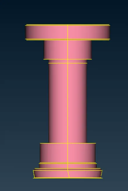
ii.) Column
The column is the component which connects the valve head to the spring, by which it is actuated up and down.
iii.) Spring
The reference force element is usually a mechanical spring. This spring exerts a force on the valve head and acts to close it. Many pressure relief valves are designed with an adjustment which allows the user to adjust the relief pressure set-point by changing the force exerted by the reference spring.
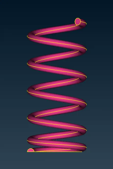
iv.) Body
It is the outer housing which encloses the various components of the pressure valve and through which the fluid enters (inlet) and exits (outlet).
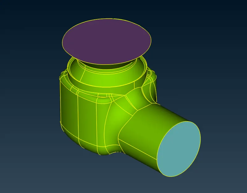
Thereby, the various PID’s of the components are assigned as follows.

3. INTERSECTION ERROR
After creating the PID’s, we need to solve the intersection error occurring due to the spring penetrating into the column.
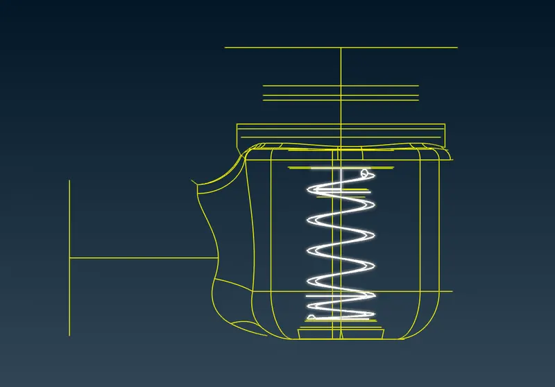
To solve this, we first use the ‘face intersect’ function, in which we define clear boundaries of the spring which is intersected with the column. Here, we select the first group as the spring and the second group as the column. From the pop-up obtained, we selected the faces to be deleted and the faces which we want to keep, respectively and thereby, solving the intersection.
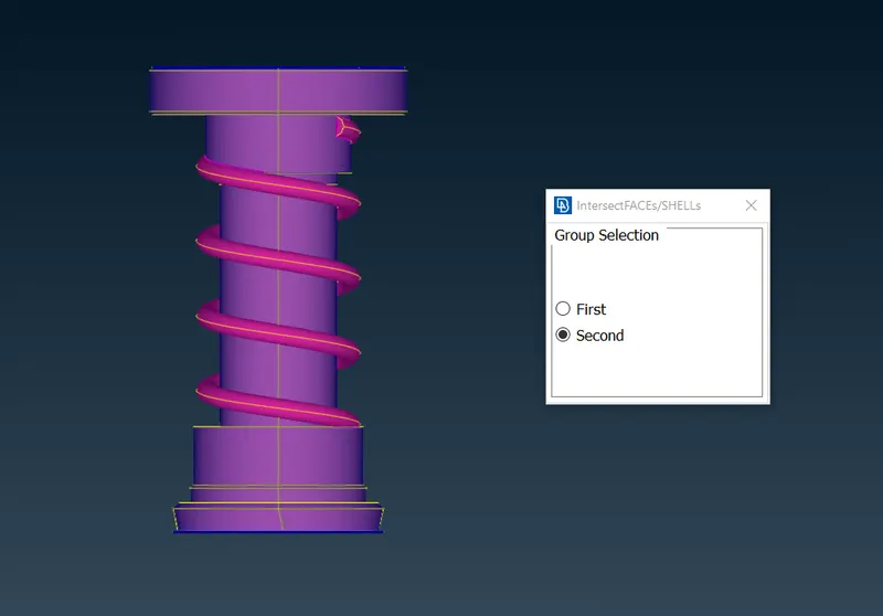
The above geometry is clear of intersections & surface errors, and we can further move on to meshing. We generate meshing for three different target lengths, i.e., 3 cases as follows.
CASE – 1 : TARGET LENGTH = 5 mm
In this case study, we are going to generate meshing of a target length of 5 mm for the pressure valve geometry.
To do this, we first assign the perimeter length and macros length as 5 mm for the geometry. This creates equally distributed points or nodes which are 5 mm apart, along the boundaries and faces of the geometry.
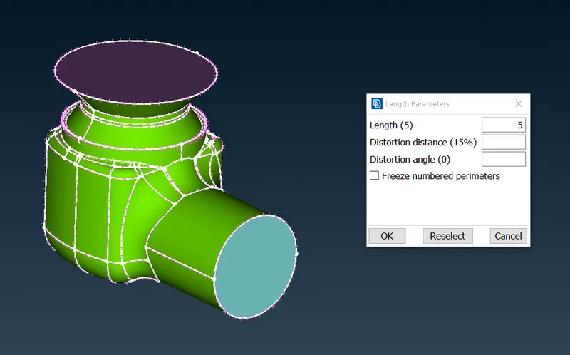
The next step is defining the quality criteria for the same. As we require a target length of 5 mm, we define the minimum length of the mesh parameter as 4 mm and maximum length as 6 mm. This makes sure that the meshing is generated within this range.
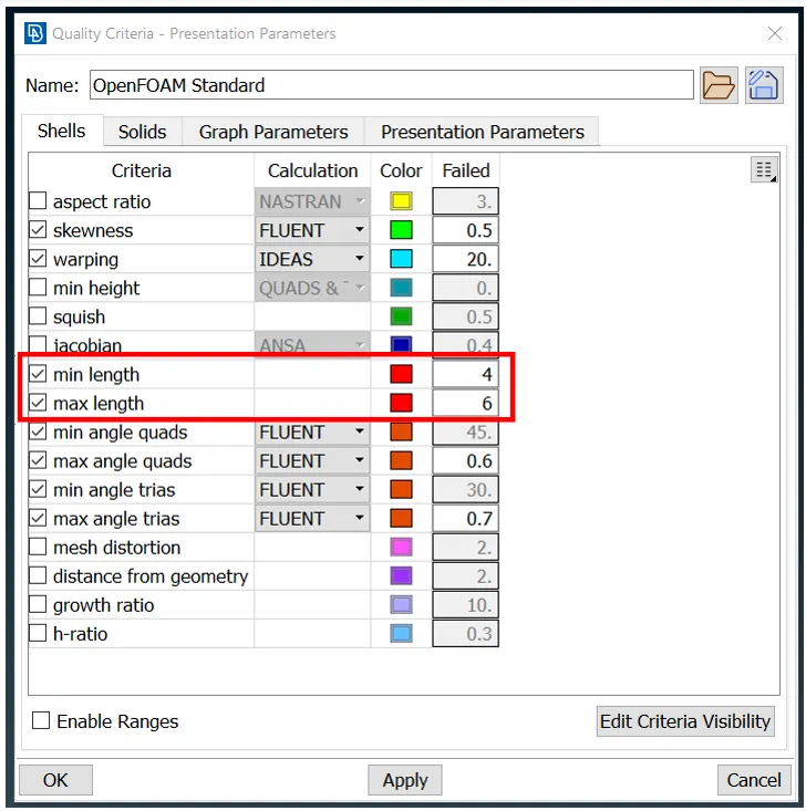
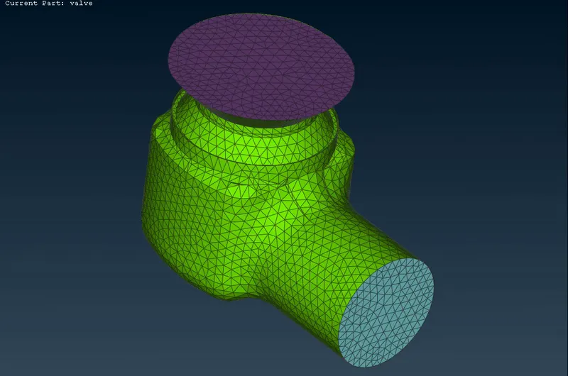
After defining the parameters and quality criteria, we finally generate Tria CFD Meshing for the entire visible geometry. We obtain a coarse mesh as shown.
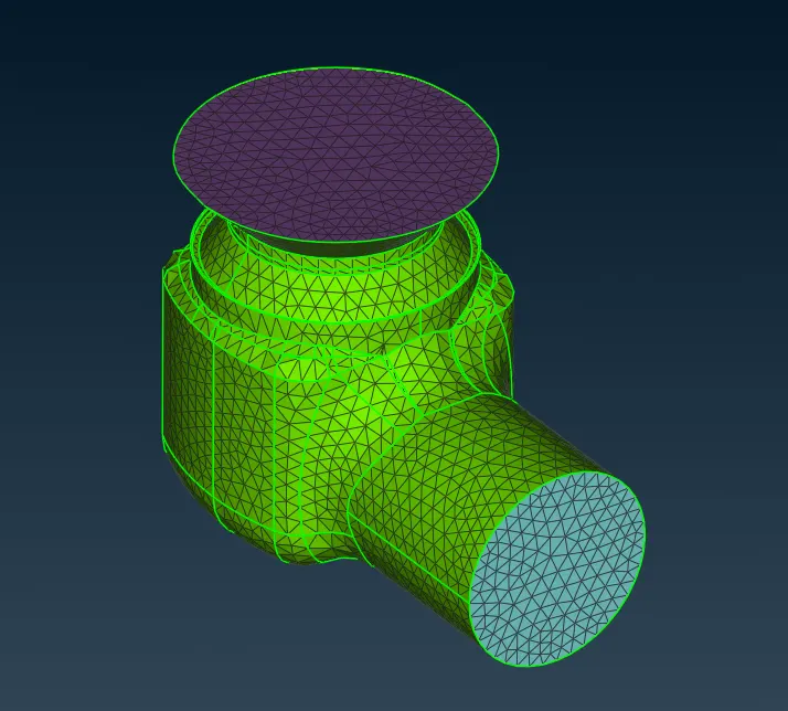
From the images shown, we can observe that the components of the pressure valve (especially the spring) have not been clearly captured, due to the high target length value. In order to capture the details more precisely, we are going to refine the meshing, in the further cases.
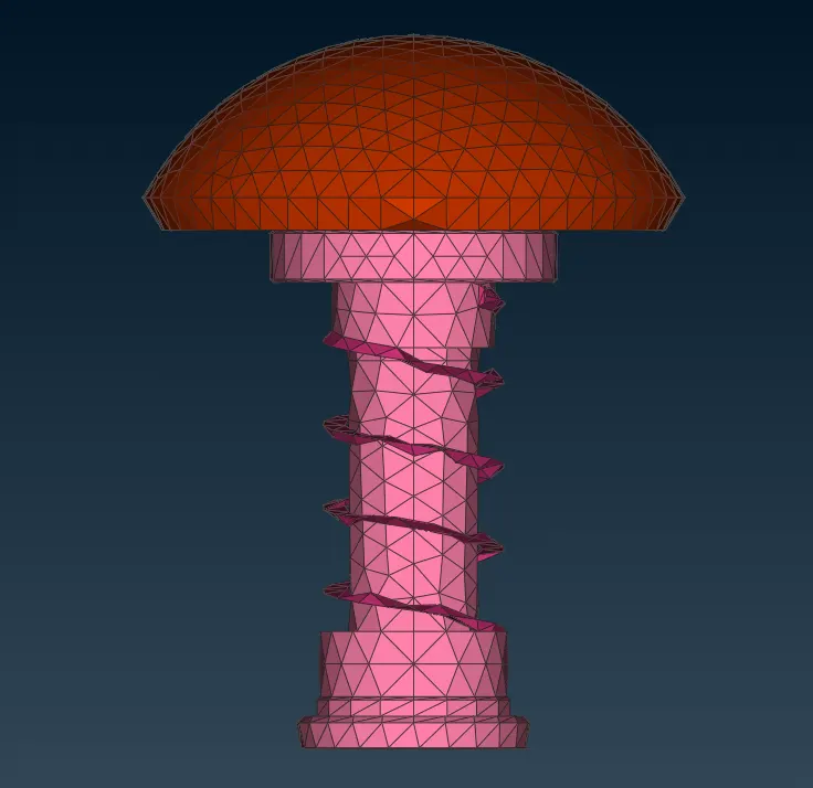
`360^o` View of the Meshed Components :
Model File : https://drive.google.com/file/d/1XuVuIdvzLXj9wA0mHwBG61cXyFaC585C/view?usp=share_link
CASE – 2 : TARGET LENGTH = 3 mm
In this case study, we are going to generate a medium refined mesh of target length 3 mm and observe the differences.
We first set the perimeter length and macros length of the geometry to 3 mm as shown.
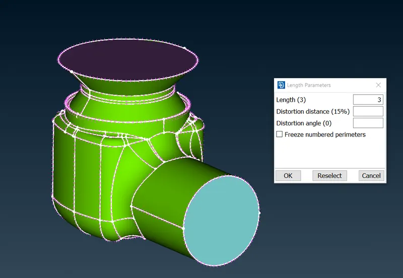
Next, we define the quality parameters of the minimum length as 2 mm and the maximum length to be 4 mm such that the generated mesh is within that range.
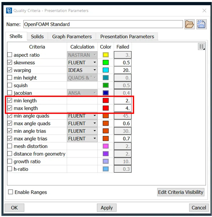
After setting the quality parameters and target lengths as shown, we finally generate the Tria CFD Meshing for the geometry as follows.
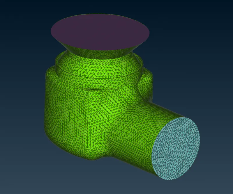
From the images, we can observe that the meshing is a bit more refined but the details of some of the components are still not perfectly captured, though it is a bit better as compared to the first case. Hence, we need to refine it more.
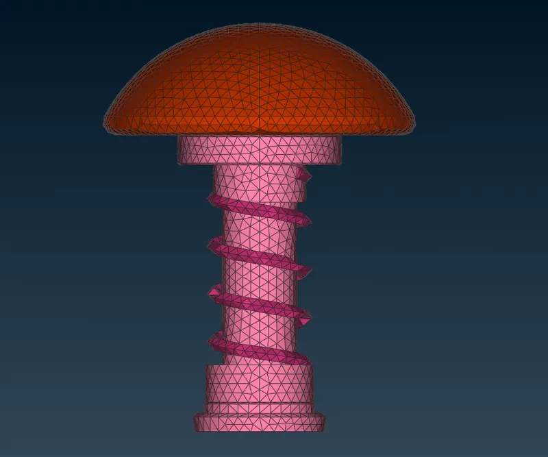
`360^o` View of the Meshed Components :
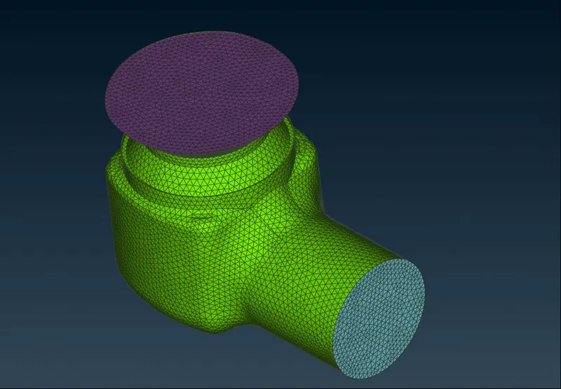
Model File : https://drive.google.com/file/d/1KhDC9pxwKD-Xohv0ceulyNoY9y854xc4/view?usp=share_link
CASE – 3 : TARGET LENGTH = 1 mm
In this final case study, we refine the mesh to a target length of 1 mm. To do so, we first set the perimeter length and macros length to a value of 1 mm as shown.
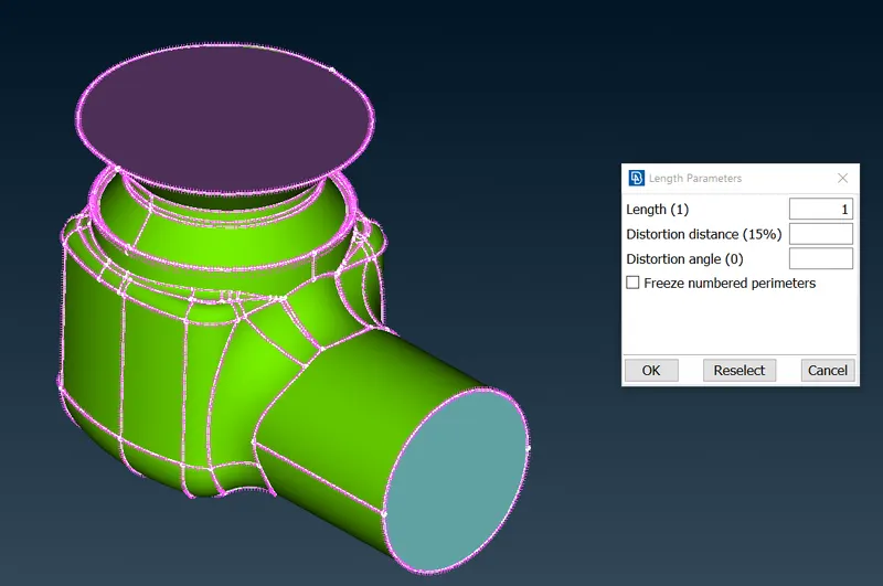
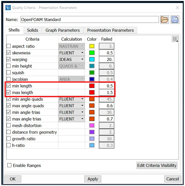
We then set the quality parameters to a minimum length of 0.5 mm and a maximum length of 1.5 mm so as to make sure the mesh length stays within that range.
Finally, we generate the Tria CFD Meshing for the geometry as shown.
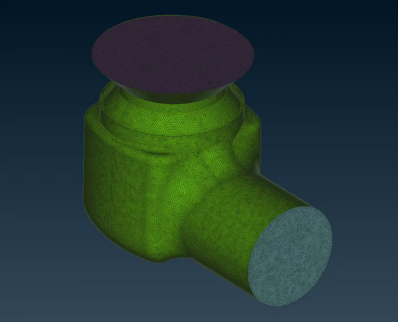
From the images, we can observe that all the details of the components such as curvatures and also the spring has been clearly captured due to the fine meshing.
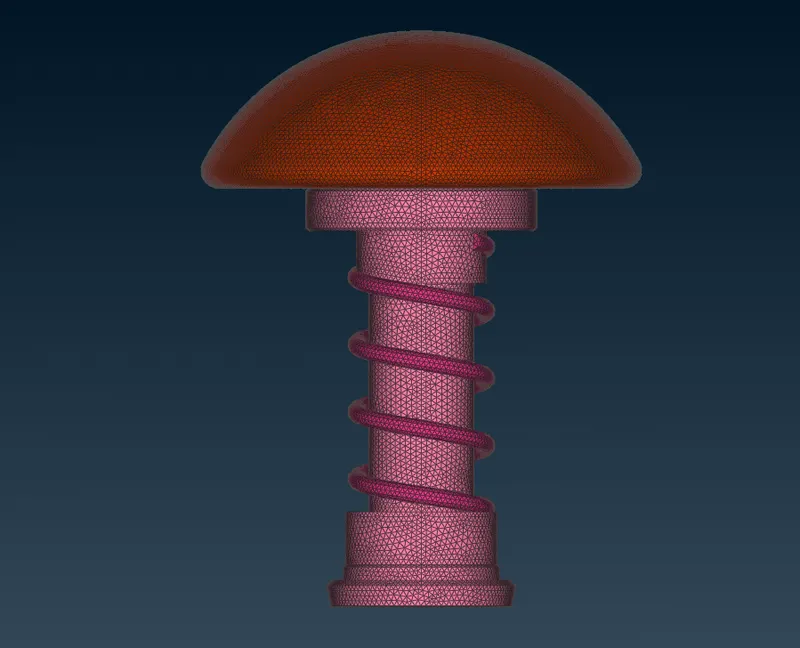
`360^o` View of the Meshed Components :
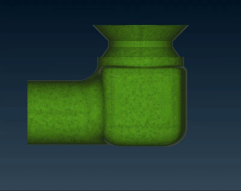
Model File : https://drive.google.com/file/d/172ZR59rw8iLzINHrtevFBfvQ7FxX0nwr/view?usp=share_link
CONCLUSIONS :
From the case studies conducted above, we can infer that as the mesh size or target length of the meshing reduces, the details of the components, such as their curvatures and spirals are captured more precisely. As we can see, when compared to target length of 5 mm, the spring component is captured more in detail by the 1 mm mesh length.
Therefore, a smaller mesh length captures finer details of the geometry. Also, as the mesh becomes more refined, the number of elements also gradually increases, which leads to an increase in computational time. Hence, finer the mesh, larger the element count.