Project 1 - Parsing NASA thermodynamic data
OBJECTIVES :
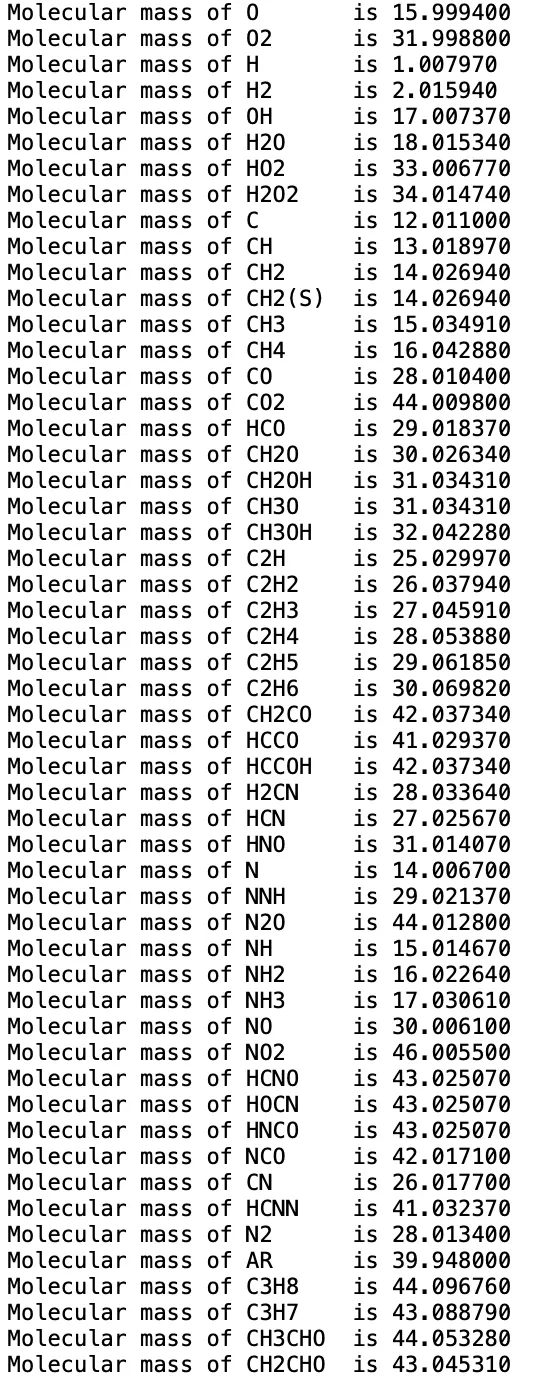
- To write a function that extracts the 14 coefficients of the NASA Thermodynamic Data file and calculate the enthalpy, entropy and specific heat for all the species in the data file.
- Calculate the molecular weight of each species and display it in the command window.
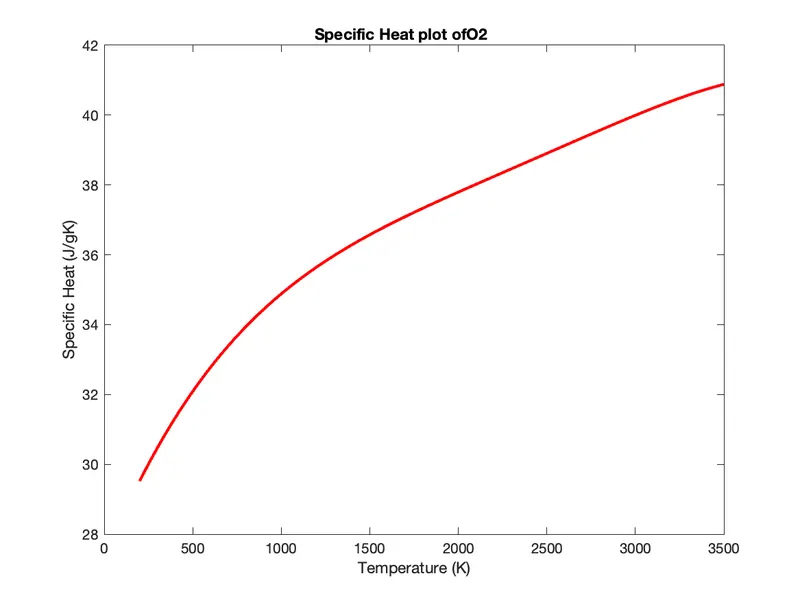
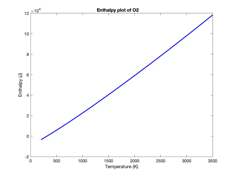
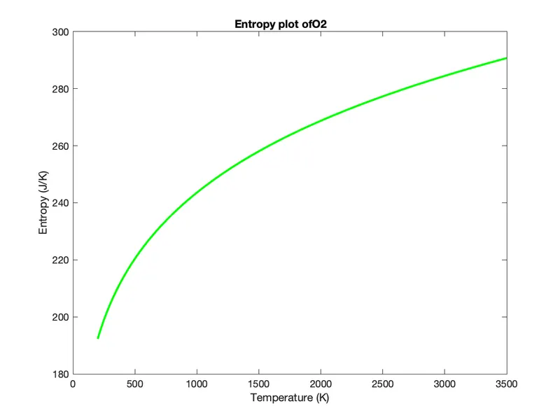
- Plot the Cp, Enthalpy and Entropy for the local temperature range (low temperature : high temperature), specific for each species.
- Write codes to automatically save the plots as images with appropriate names and dumping them into separate folders for each species.
- Write the program in such a way that it takes “THERMO.dat” file as an input and generates Cp, H and S as plots.
INTRODUCTION :
Parsing is the process of converting formatted text into a data structure. The File Parser process enables us to read data from an external file or database and place it into tables or include that data in calculations. The external file can be a delimited file or a flat file. It can be a simple file with one row type or a complex file with several row types.

The above figure represents a simple example of file parsing from a string (source) in the format DD-MM-YYYY.
TERMS :
1. Specific Heat (Cp)
Specific heat is defined as the the heat required to raise the temperature of the unit mass of a given substance by a given amount (usually one degree).
The units are often Joules per gram-degree Celsius (J/g °C).
2. Enthalpy (H)
Enthalpy is a thermodynamic quantity equivalent to the total heat content of a system. It is equal to the internal energy of the system plus the product of pressure and volume.
The units of enthalpy are in J or kJ.
3. Entropy (S)
Entropy is a thermodynamic quantity representing the unavailability of a system's thermal energy for conversion into mechanical work, often interpreted as the degree of disorder or randomness in the system.
The units of entropy are J/K.
4. Molecular Weight (MW)
Molecular weight is defined as the sum of atomic weights of atoms in a molecule. It is also referred to as molecular mass.
The base SI unit for molecular weight is kg/mole and are also expressed in gm/mole.
GOVERNING EQUATIONS :
The formulas involved in the calculations are as follows.
- Specific Heat
`(C_p)/R = a_1 + a_2 T + a_3 T^2 + a_4T^3 + a_5T^4` - Enthalpy
`H/(RT) = a_1 + (a_2T)/2 + (a_3T^2)/3 + (a_4T^3)/4 + (a_5T^4)/5 + a_6/T` - Entropy
`S/R = a_1 lnT + a_2T + (a_3T^2)/2 + (a_4T^3)/3 + (a_5T^4)/4 + a_7`
Where,
Cp = Specific Heat of the system (J/gK)
H = Enthalpy (J or kJ)
S = Entropy (J/K)
R = Universal Gas Constant = 8.314 J/mol.K
T = Temperature (K)
DETAILED PROCEDURE AND EXPLANATION :
Step – 1 :
We begin the program by using clear all, close all and clc commands to clear up the workspace as well as the command window.
In the next step, we read the data from the external file ‘THERMO.dat’ containing the useful data which is to be parsed. This external file is to be saved in the same file directory in which the program is saved.
The contents of the file are read by using the ‘fopen’ command and the contents of which are assigned to a variable or file handle ‘f1’. ‘r’ denotes reading the file.
Another text file under the name ‘molecular mass.txt’ is created, which is a text file in which all the data of the calculated molecular mass is written and is assigned to a variable ‘f2’. ‘w’ denotes writing the file.
Code :
% NASA Thermodynamic Data Parsing
clear all
close all
clc

% opening and reading the data file
f1 = fopen('THERMO.dat','r')

% creating text file to save molecular mass data
f2 = fopen('molecular mass.txt','w')
Step – 2 :
The next step involves extracting information from the first 5 lines of the file. We use the ‘fgetl’ command to read the file line by line. By running the fgetl command for a second time, we get the next line and so on.
The first line of the data file is the heading. By using the fgetl(f1) command, we extract the first line and assign it to a character ‘heading’
The second line of the file is the global temperature range. We use the ‘strsplit’ command to split the string at a specified delimiter, which in this case, is a space. The ‘str2double’ command is used to convert the cell array into a numerical array of the same size. Thereby, we extract the global low, mid and high temperatures.
As the next three lines of the file are comments, we skip past through it by using the fgetl command, as they have no significant value.
Code :
% PART - 1
% extracting the header information
% heading of the file
heading = fgetl(f1)

% processing global temperature data
global_temperature_range = fgetl(f1)

% extracting global low, mid and high temperatures from global temperature
a = strsplit(global_temperature_range,' ')
global_temperature = str2double(a)

global_low_temperature = global_temperature(2)
global_medium_temperature = global_temperature(3)
global_high_temperature = global_temperature(4)


% running past the three comment lines
comment_1 = fgetl(f1)
comment_2 = fgetl(f1)
comment_3 = fgetl(f1)
Step – 3 :
The next step involves extracting the species name, their local temperatures and their coefficients. There are a total of 53 species of elements in the data file. We use a for loop command to get the individual data of each species.
To extract the name of the species, we use the ‘findstr’ command to locate the space which is present after each species name and by using the range operator ‘species_line_1 (1 : c(1)+5)’, we obtain the exact location of the species names.
Similarly, to extract the local temperature values, we use ‘findstr’ command as well to locate the decimal point located in each temperature value. As the value obtained will be in the form of a string, we change it to a numerical value by using ‘str2num’ command. Therefore we obtain the values for local low, mid and high temperature for each species.
Finally, using the same logic, we use ‘findstr’ command and locate all the positions of string ‘E’ in the next three lines of species data and by using the range operators, we accurately locate and determine all 14 coefficients of the species.
Code :
% extracting data of each species
% there are a total of 53 species in data file
for i = 1:53

    % extracting name of species
    species_line_1 = fgetl(f1)
    c = findstr(species_line_1,' ')
    species_name = species_line_1(1:c(1)+5)


    % extracting local temperature of species
    d = findstr(species_line_1,'.')

    t1 = species_line_1((d(1)-3):(d(1)+4))
    local_low_temperature = str2num(t1)

    t2 = species_line_1((d(2)-4):(d(2)+4))
    local_high_temperature = str2num(t2)

    t3 = species_line_1((d(3)-4):(d(3)+4))
    local_mid_temperature = str2num(t3)


    % extracting the 14 coefficients of the species
    % species line 2
    species_line_2 = fgetl(f1)
    d = findstr(species_line_2,'E')

    A1 = species_line_2((d(1)-11):(d(1)+3))
    a1 = str2num(A1)

    A2 = species_line_2((d(1)+4):(d(2)+3))
    a2 = str2num(A2)

    A3 = species_line_2((d(2)+4):(d(3)+3))
    a3 = str2num(A3)

    A4 = species_line_2((d(3)+4):(d(4)+3))
    a4 = str2num(A4)

    A5 = species_line_2((d(4)+4):(d(5)+3))
    a5 = str2num(A5)


    % species line 3
    species_line_3 = fgetl(f1)
    e = findstr(species_line_3,'E')

    A6 = species_line_3((e(1)-11):(e(1)+3))
    a6 = str2num(A6)

    A7 = species_line_3((e(1)+4):(e(2)+3))
    a7 = str2num(A7)

    A8 = species_line_3((e(2)+4):(e(3)+3))
    a8 = str2num(A8)

    A9 = species_line_3((e(3)+4):(e(4)+3))
    a9 = str2num(A9)

    A10 = species_line_3((e(4)+4):(e(5)+3))
    a10 = str2num(A10)


    % species line 4
    species_line_4 = fgetl(f1)
    f = findstr(species_line_4,'E')

    A11 = species_line_4((f(1)-11):(f(1)+3))
    a11 = str2num(A11)

    A12 = species_line_4((f(1)+4):(f(2)+3))
    a12 = str2num(A12)

    A13 = species_line_4((f(2)+4):(f(3)+3))
    a13 = str2num(A13)

    A14 = species_line_4((f(3)+4):(f(4)+3))
    a14 = str2num(A14)
Where, a1 – a7 are coefficients for high temperature range and a8 – a14 are coefficients for low temperature range.
Step – 4 :
The next step involves calculating the specific heat, enthalpy and entropy for all the species by using the formulas shown below:

In order to calculate that, we first define the temperature range ‘T’. If the temperature value is in the local high temperature range, we substitute the coefficients a1 – a7 in the above formulas and if the temperature value is in the local low temperature range, we use the coefficients a8 – a14 and thereby obtain the values for specific heat, enthalpy and entropy.
Code :
    % PART - 2
    % calculating values of specific heat, enthalpy and entropy
    % defining range of temperatures
    T = linspace(local_low_temperature,local_high_temperature,500);

    % universal gas constant (J/mol.K)
    R = 8.314

    for j = 1:length(T)
        if T(j)>local_mid_temperature

            % specific heat for high temperature range
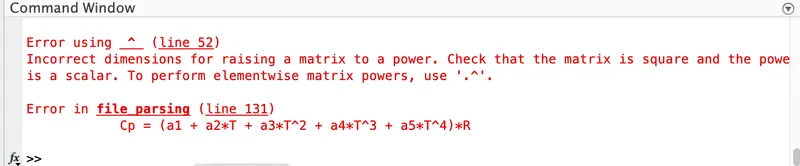
            Cp = (a1 + a2*T + a3*T.^2 + a4*T.^3 + a5*T.^4)*R

            % enthalpy for high temperature range
            H = (a1 + ((a2.*T)./2) + ((a3.*(T.^2))./3) + ((a4.*(T.^3))./4) + ((a5.*(T.^4))./5) + (a6./T))*R.*T

            % entropy for high temperature range
            S = ((a1*log(T)) + (a2*T) + ((a3*(T.^2))/2) + ((a4*(T.^3))/3) + ((a5*(T.^4))/4) + a7)*R

        else
            % specific heat for low temperature range
            Cp = (a8 + a9*T + a10*T.^2 + a11*T.^3 + a12*T.^4)*R

            % enthalpy for low temperature range
            H = (a8 + ((a9.*T)./2) + ((a10.*(T.^2))./3) + ((a11.*(T.^3))./4) + ((a12.*(T.^4))./5) + (a13./T))*R.*T

            % entropy for low temperature range
            S = ((a8.*log(T)) + (a9.*T) + ((a10.*(T.^2))./2) + ((a11.*(T.^3))./3) + ((a12.*(T.^4))./4) + a14)*R
        end
    end
Step – 5 :
In this step, we calculate the molecular weight of each individual species and display the results in the file ‘f2’, which is the molecular weight text file.
In order to do so, we first determine the elements which are repeated as a combination in all 53 of the element species. We define these elements as an array and we define the respective atomic weights for these elements in a different array. We declare the initial molecular weight as 0.
We use the ‘strcmp’ command to compare the species name with the elements array and the atomic weight is added with reference to the compared string value elements.
We find the repetition of elements of same species by extracting a variable ‘n’ using ‘str2double’ command. If the species name, which is now a number, is greater than 1, the molecular weight is calculated again by multiplying the atomic weights with a factor of (n-1).
We then use the ‘fprintf’ command to display the results of molecular weights of all the species in the file ‘f2’.
Code :
    % PART - 3
    % calculating the molecular weight of each species
    % defining elements
    elements = ['O','H','C','N','A']

    % assigning atomic weights to elements array
    atomic_weights = [15.9994,1.00797,12.011,14.0067,39.948]

    % initializing molecular weight value
    molecular_weight = 0

    for l = 1:length(species_name)
        for m = 1:length(atomic_weights)

            if strcmp(species_name(l),elements(m))
                molecular_weight = molecular_weight + atomic_weights(m)
                p = m
            end
        end

        n = str2double(species_name(l));

        if n>1
            molecular_weight = molecular_weight + atomic_weights(p)*(n-1)
        end
    end


    % writing a file with molecular weight data
    fprintf(f2,'Molecular mass of %s is %f\n',species_name,molecular_weight)
Step – 6 :
The last and final step in this program is plotting all the data of specific heat, enthalpy and entropy against temperature for all the species and creating a separate folder so as to dump all the data into it such that it contains individual folders of the species with its graphs stored in it.
To do so, we first create a new folder of the species names, in our file directory using the ‘mkdir’ command. Next, we use the ‘cd’ command to change the file directory from the main folder to the species names folder.
Finally, we plot the graphs of specific heat, enthalpy and entropy on the y-axes against temperature on the x-axis, for all the species. We then use the ‘saveas’ command to save these plots in their individual folders.
Code :
    % PART - 4
    % creating folder to save the plots
    mkdir('Plot_Data',species_name)

    % changing folder directory
    cd('Plot_Data')

    % plotting graphs of specific heat, enthalpy and entropy
    % plotting specific heat for local temperature range
    figure(1)
    plot(T,Cp,'LineWidth',2,'Color','r')
    title(['Specific Heat plot of',species_name])
    xlabel('Temperature (K)')
    ylabel('Specific Heat (J/gK)')
    saveas(figure(1),'Specific Heat.png')

    % plotting enthalpy for local temperature range
    figure(2)
    plot(T,H,'LineWidth',2,'Color','b')
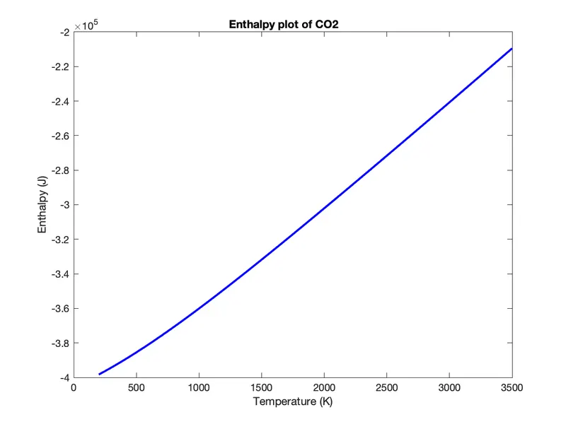
    title(['Enthalpy plot of ',species_name])
    xlabel('Temperature (K)')
    ylabel('Enthalpy (J)')
    saveas(figure(2),'Enthalpy.png')

    % plotting entropy for local temperature range
    figure(3)
    plot(T,S,'LineWidth',2,'Color','g')
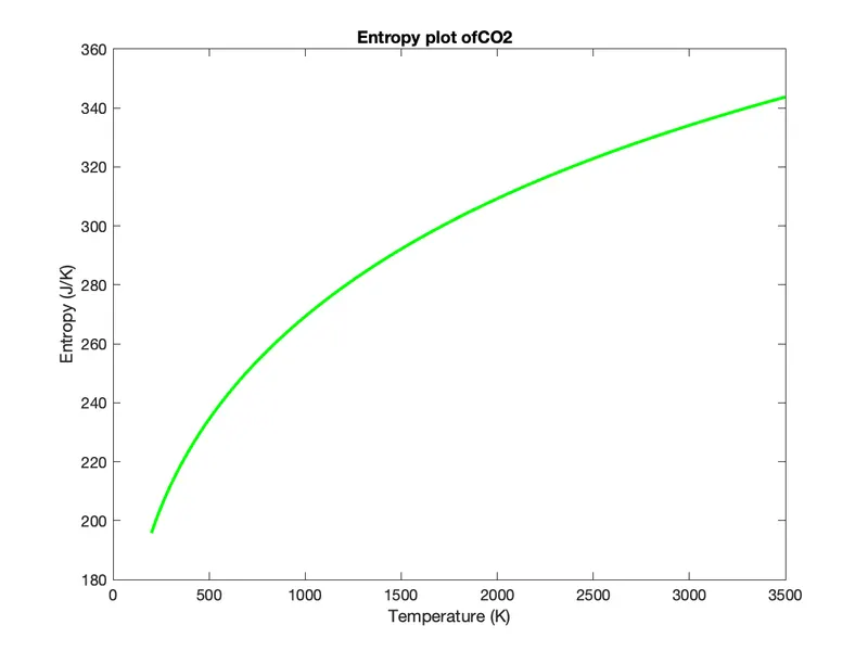
    title(['Entropy plot of',species_name])
    xlabel('Temperature (K)')
    ylabel('Entropy (J/K)')
    saveas(figure(3),'Entropy.png')
end

fclose(f2)
fclose(f1)
FINAL PROGRAM CODE :
% NASA Thermodynamic Data Parsing
clear all
close all
clc

% opening and reading the data file
f1 = fopen('THERMO.dat','r')

% creating text file to save molecular mass data
f2 = fopen('molecular mass.txt','w')

% PART - 1
% extracting the header information
% heading of the file
heading = fgetl(f1)

% processing global temperature data
global_temperature_range = fgetl(f1)

% extracting global low, mid and high temperatures from global temperature
a = strsplit(global_temperature_range,' ')
global_temperature = str2double(a)

global_low_temperature = global_temperature(2)
global_medium_temperature = global_temperature(3)
global_high_temperature = global_temperature(4)


% running past the three comment lines
comment_1 = fgetl(f1)
comment_2 = fgetl(f1)
comment_3 = fgetl(f1)


% extracting data of each species
% there are a total of 53 species in data file
for i = 1:53

    % extracting name of species
    species_line_1 = fgetl(f1)
    c = findstr(species_line_1,' ')
    species_name = species_line_1(1:c(1)+5)


    % extracting local temperature of species
    d = findstr(species_line_1,'.')

    t1 = species_line_1((d(1)-3):(d(1)+4))
    local_low_temperature = str2num(t1)

    t2 = species_line_1((d(2)-4):(d(2)+4))
    local_high_temperature = str2num(t2)

    t3 = species_line_1((d(3)-4):(d(3)+4))
    local_mid_temperature = str2num(t3)


    % extracting the 14 coefficients of the species
    % species line 2
    species_line_2 = fgetl(f1)
    d = findstr(species_line_2,'E')

    A1 = species_line_2((d(1)-11):(d(1)+3))
    a1 = str2num(A1)

    A2 = species_line_2((d(1)+4):(d(2)+3))
    a2 = str2num(A2)

    A3 = species_line_2((d(2)+4):(d(3)+3))
    a3 = str2num(A3)

    A4 = species_line_2((d(3)+4):(d(4)+3))
    a4 = str2num(A4)

    A5 = species_line_2((d(4)+4):(d(5)+3))
    a5 = str2num(A5)


    % species line 3
    species_line_3 = fgetl(f1)
    e = findstr(species_line_3,'E')

    A6 = species_line_3((e(1)-11):(e(1)+3))
    a6 = str2num(A6)

    A7 = species_line_3((e(1)+4):(e(2)+3))
    a7 = str2num(A7)

    A8 = species_line_3((e(2)+4):(e(3)+3))
    a8 = str2num(A8)

    A9 = species_line_3((e(3)+4):(e(4)+3))
    a9 = str2num(A9)

    A10 = species_line_3((e(4)+4):(e(5)+3))
    a10 = str2num(A10)


    % species line 4
    species_line_4 = fgetl(f1)
    f = findstr(species_line_4,'E')

    A11 = species_line_4((f(1)-11):(f(1)+3))
    a11 = str2num(A11)

    A12 = species_line_4((f(1)+4):(f(2)+3))
    a12 = str2num(A12)

    A13 = species_line_4((f(2)+4):(f(3)+3))
    a13 = str2num(A13)

    A14 = species_line_4((f(3)+4):(f(4)+3))
    a14 = str2num(A14)

    % where a1 - a7 are coefficients of high temperature
    % and a8 - a14 are coefficients of low temperature


    % PART - 2
    % calculating values of specific heat, enthalpy and entropy
    % defining range of temperatures
    T = linspace(local_low_temperature,local_high_temperature,500);

    % universal gas constant (J/mol.K)
    R = 8.314

    for j = 1:length(T)
        if T(j)>local_mid_temperature

            % specific heat for high temperature range
            Cp = (a1 + a2*T + a3*T.^2 + a4*T.^3 + a5*T.^4)*R

            % enthalpy for high temperature range
            H = (a1 + ((a2.*T)./2) + ((a3.*(T.^2))./3) + ((a4.*(T.^3))./4) + ((a5.*(T.^4))./5) + (a6./T))*R.*T

            % entropy for high temperature range
            S = ((a1*log(T)) + (a2*T) + ((a3*(T.^2))/2) + ((a4*(T.^3))/3) + ((a5*(T.^4))/4) + a7)*R

        else
            % specific heat for low temperature range
            Cp = (a8 + a9*T + a10*T.^2 + a11*T.^3 + a12*T.^4)*R

            % enthalpy for low temperature range
            H = (a8 + ((a9.*T)./2) + ((a10.*(T.^2))./3) + ((a11.*(T.^3))./4) + ((a12.*(T.^4))./5) + (a13./T))*R.*T

            % entropy for low temperature range
            S = ((a8.*log(T)) + (a9.*T) + ((a10.*(T.^2))./2) + ((a11.*(T.^3))./3) + ((a12.*(T.^4))./4) + a14)*R
        end
    end


    % PART - 3
    % calculating the molecular weight of each species
    % defining elements
    elements = ['O','H','C','N','A']

    % assigning atomic weights to elements array
    atomic_weights = [15.9994,1.00797,12.011,14.0067,39.948]

    % initializing molecular weight value
    molecular_weight = 0

    for l = 1:length(species_name)
        for m = 1:length(atomic_weights)

            if strcmp(species_name(l),elements(m))
                molecular_weight = molecular_weight + atomic_weights(m)
                p = m
            end
        end

        n = str2double(species_name(l));

        if n>1
            molecular_weight = molecular_weight + atomic_weights(p)*(n-1)
        end
    end

    % printing molecular weight of species in command window
    sprintf('Molecular Weight of %s is %f',species_name,molecular_weight)


    % PART - 4
    % creating folder to save the plots
    mkdir('Plot_Data',species_name)

    % changing folder directory
    cd('Plot_Data')

    % plotting graphs of specific heat, enthalpy and entropy
    % plotting specific heat for local temperature range
    figure(1)
    plot(T,Cp,'LineWidth',2,'Color','r')
    title(['Specific Heat plot of',species_name])
    xlabel('Temperature (K)')
    ylabel('Specific Heat (J/gK)')
    saveas(figure(1),'Specific Heat.png')

    % plotting enthalpy for local temperature range
    figure(2)
    plot(T,H,'LineWidth',2,'Color','b')
    title(['Enthalpy plot of ',species_name])
    xlabel('Temperature (K)')
    ylabel('Enthalpy (J)')
    saveas(figure(2),'Enthalpy.png')

    % plotting entropy for local temperature range
    figure(3)
    plot(T,S,'LineWidth',2,'Color','g')
    title(['Entropy plot of',species_name])
    xlabel('Temperature (K)')
    ylabel('Entropy (J/K)')
    saveas(figure(3),'Entropy.png')


    % writing a file with molecular weight data
    fprintf(f2,'Molecular mass of %s is %f\n',species_name,molecular_weight)
end

fclose(f2)
fclose(f1)
OUTPUT PLOTS :
1. Window where all the species folders are saved.

2. Text file in which the molecular weight of all the species is printed.
3. Output plots of specific heat, enthalpy and entropy.
Plots of O2 :
Plots for N2 :
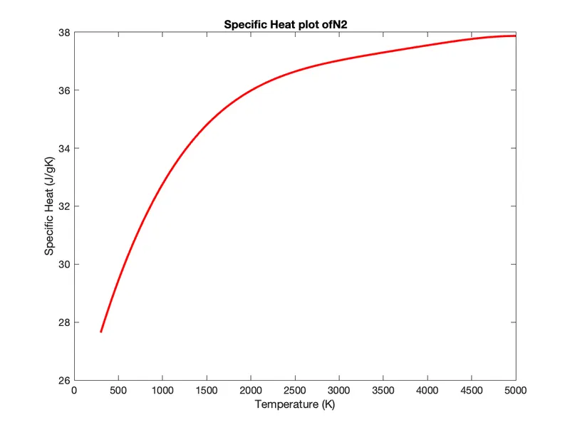
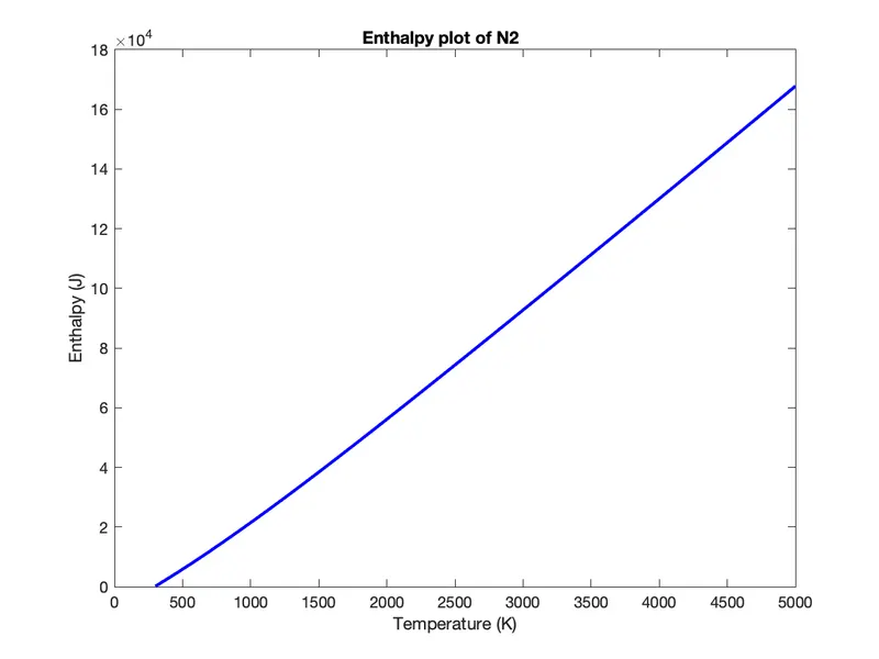
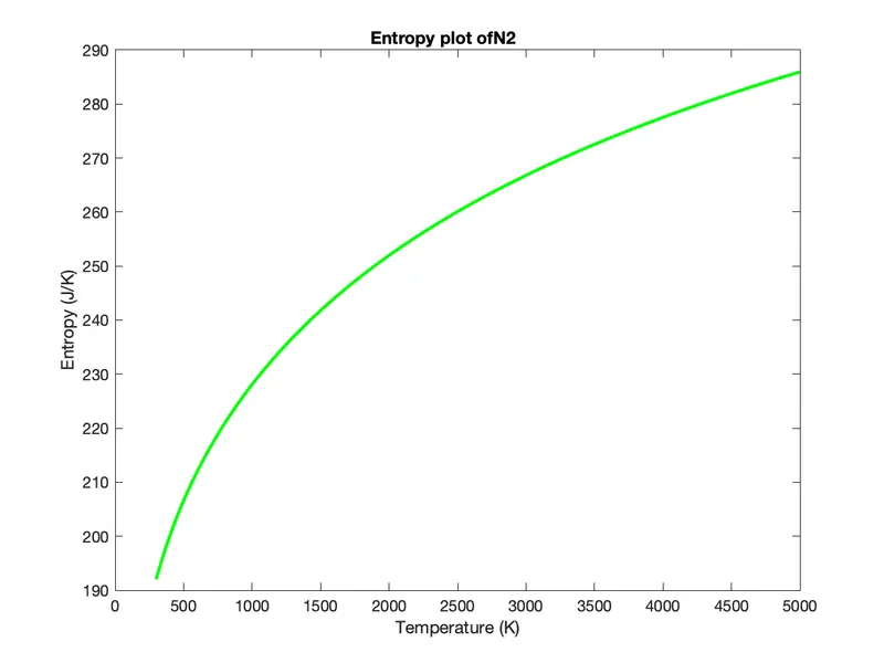
Plots for CO2 :
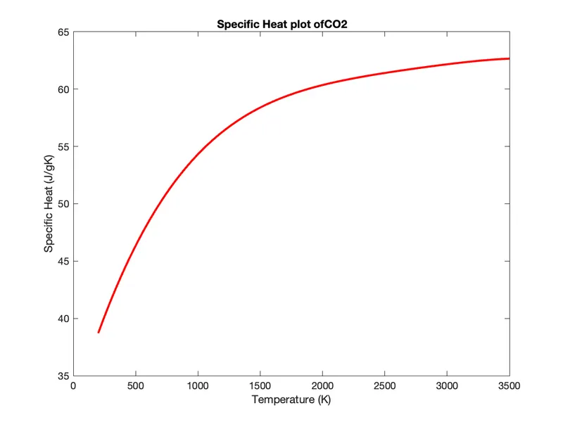
PROBLEMS ENCOUNTERED :
- While defining the formula for the specific heat calculation, I did not use the dot product operator, as a result of which I obtained a vector multiplication error.
Supposed to be:

Mistake :

Output result :
2. Encountered a few errors while using the 'cd' function as i was a bit confused regarding the file directories but were later sorted out.
CONCLUSION :
- The program to parse the given file has been written and the 14 coefficients of each species have been extracted for the local temperature range.
- The specific heat, enthalpy and entropy for all the species have been calculated and the plots have been separately saved in a folder under the name ‘Plot_Data’ automatically by taking the file ‘THERMO.dat’ as the input.
- The molecular weights of all the species have been calculated as well and are displayed in a text file under the name ‘molecular mass.txt’.
- The related outputs and observations have been displayed in the report in detail and thereby, the program is complete.
REFERENCES :
https://en.wikipedia.org/wiki/Parsing