Week 3 - Solving second order ODEs

OBJECTIVES :

Write a program in Matlab / Octave that will simulate the motion of a simple pendulum.

INTRODUCTION :

A simple pendulum is a body suspended from a fixed point so it can swing back and forth under the influence of gravity. Pendulums, like masses on a spring, are examples of simple harmonic oscillators.

It consists of a small bob of mass ‘m’ suspended at the end of a thread of length ‘L’ that is so light as to be considered massless. The period of such a device can be made longer by increasing its length, as measured from the point of suspension to the middle of the bob. A change in the mass of the bob, however, does not affect the period, provided the length is not thereby affected.

Assumptions:

• There is negligible friction from the air and the system
• The arm of the pendulum does not bend or compress and is massless
• The pendulum swings in a perfect plane
• Gravity remains constant.

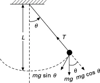
A pendulum's bob swinging is kept in motion by the force acting upon it as it moves back and forth. In pendulum motion, three forces work directly on the pendulum​: the mass of the bob, gravity and the tension in the string. Mass and gravity both work vertically downward. Since the pendulum doesn’t move up or down, the vertical component of the string tension cancels out the mass and gravity.

This shows that the mass of a pendulum has no relevance to its motion, but the horizontal string tension does.

GOVERNING EQUATIONS :

The Ordinary Differential Equation (ODE) that represents the motion of a simple pendulum is given by,

`(d^2theta)/(dt^2) + b/m (d theta)/dt + g/L sin theta = 0`

Where, b = damping coefficient

m = mass of the pendulum bob

g = gravitational constant

L = length of massless string or rod

`theta`= angle of pendulum

By solving the above equation, we are solving for '`theta`' and rate at which `theta` value is changing with respect to time, which is nothing but velocity.

The first and foremost fundamental of solving this equation is breaking down the higher order ODE's into a set of first order ODE's.

As we know, `(d^2 theta)/dt^2` is a second order ODE.

To transform this second order ODE to a first order ODE,

Considering, `theta = theta_1`

Therefore, `(d theta)/dt = (d theta_1)/dt = theta_2` - equation (1)

Also, `(d^2 theta)/dt^2 = (d^2 theta_1)/dt^2` `{because theta = theta_1}`

`(d^2 theta)/dt^2 = d/dt((d theta_1)/dt)`

From equation (1),

`(d^2 theta)/dt^2 = d/dt (theta_2)` - equation (2)

If `theta = theta_1`, the simple pendulum equation becomes,

`(d^2theta_1)/(dt^2) + b/m (d theta_1)/dt + g/L sin theta_1 = 0`

Therefore, from equation (1) and equation (2),

`(d theta_2)/(dt) + b/m (theta_2) + g/L sin theta_1 = 0`

This means that, to solve the original second order ODE, we have created two ODE's, thereby breaking down the second order ODE into series of first order ODE's.

That is, `(d theta_1)/dt = theta_2` and `(d theta_2)/(dt) = - b/m (theta_2) - g/L sin theta_1`

Therefore, in matrix form, the solution vector is given by,

`d/(dt) [(theta_1), (theta_2)] = [(theta_2),(-b/m theta_2 - g/L sintheta_1)]`

DETAILED PROCEDURE AND EXPLANATION :

The various steps involved in writing a program to animate the motion of a simple pendulum are as follows.

Step – 1 :

The first and foremost step involved in solving the ODE begins by breaking the 2^nd order ODE into a set of 1^st order ODE’s. Thereby, we obtain the two equations as follows:

`(d theta_1)/dt = theta_2` and `(d theta_2)/(dt) = - b/m (theta_2) - g/L sin theta_1`

After transforming the 2^nd order equation into the above mentioned 1^st order equations, we further move on to define the input variables. The input variables are as follows,

1. Damping coefficient b = 0.05
2. Mass of the pendulum bob m = 1 kg
3. Gravitational constant g = 9.81 m/s²
4. Length of pendulum l = 1 m

Code:

% inputs
% damping coefficient
b = 0.05

% mass of bob (kg)
m = 1

% gravitational constant (m/s²)
g = 9.81

% length of pendulum (m)
l = 1

Step – 2 :

After defining the inputs as represented above, we then define the initial conditions and time span arrays for the system.

As mentioned in the problem, the angular displacement and angular velocity of the pendulum at t = 0 is “0” and “3 rad/sec” respectively, they are considered to be the initial conditions of the system.

And also, as we need to simulate the motion of the pendulum between 0 – 20 seconds, we consider that as the time span.

Code:

% initial conditions
% theta_0 = [angular_displacement ; angular_velocity]
theta_0 = [0;3]

% time span
% pendulum oscillates between 0 to 20 seconds
t_span = linspace(0,20,500);

Step – 3 :

Before heading further, we need to define `(d theta)/dt` as a function of t , theta , b , m , g and l respectively.

As we have already transformed the 2nd order ODE into a set of 1st order equations, we obtain the function code as follows.

Code:

% defining ODE45 function
function [dtheta_dt] = ode_function(t,theta,b,m,g,l)
theta1 = theta(1)
theta2 = theta(2)
dtheta1_dt = theta2
dtheta2_dt = -(b/m)*theta2 - (g/l)*sin(theta1)
dtheta_dt = [dtheta1_dt;dtheta2_dt]
end

Step – 4 :

The next step involves solving the “ode45” equation with respect to the defined function. The ode45 function contains 3 inputs, being the function to be integrated, the time span considered and the initial conditions of the system.

Defining the function as “[ t , results ]” refers to the results being solved as a function of time.

Code:

% solving ODE equation
[t,results] = ode45(@(t,theta) ode_function(t,theta,b,m,g,l),t_span,theta_0)

Step – 5 :

The obtained results are then plotted as a graph showing the damped motion of the simple pendulum. It contains two plots, one displaying angular displacement and the other displaying angular velocity, both with respect to time.

Output Graph :

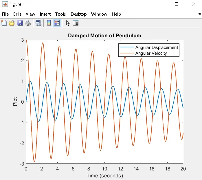
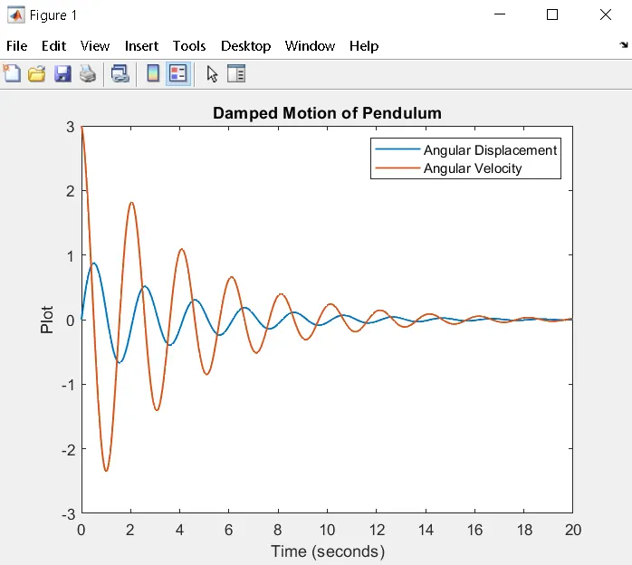
By increasing the value of damping coefficient, we obtain a smoother graph in which the vibrations are damped, corresponding to the particular damping coefficient.

For example, for the value of b = 0.5, we obtain the graph as follows.

Step – 6 :

The next step involves forming a “for loop function” to create a looping animation plot describing the motion of the pendulum. In order to do that, a loop counter “i” is first assigned for the looping function so as to determine how many times the loop is going to be executed. And also, a counter “ct” is added before the for loop which increments each step by a value of 1 (ct + 1) in every iteration of the loop.

After defining the loop counter, we further assign the values for the coordinates x0 , x1 , y0 and y1 respectively.

Code:

% for loop function
ct = 1;
for i = 1:length(results(:,1));
    x0 = 0
    y0 = 0

    x1 = l*sin(results(i));
    y1 = -l*cos(results(i));

Step – 7 :

The final step in this program involves plotting the coordinates so as to obtain an animation representing the motion of the pendulum and to create a movie file of the same.

In order to do that, let us first consider three steps to plot the graph.

1. First we need to plot the coordinates ([ -1 1 ] , [ 0 0 ]) to obtain the fixed platform or line to which the pendulum is fixed.
   
   

   plot([-1 1],[0 0],'LineWidth',4,'color','b')​

2. Next, we plot the coordinates of ([ x0 x1 ] , [ y0 y1 ]) to obtain the motion of the string or the masless rod of the pendulum. Where x0 and y0 are the points fixed to the platform and x1 and y1 are the different positions of the bob at respective time intervals.
   
   

    plot([x0 x1],[y0 y1],'LineWidth',3,'Color','y')​

3. To create the bob, we use a marker function and on that note, we fix the axes to a required range to get the animation of the pendulum motion.
   
   

   plot(x1,y1,'Marker','O','MarkerSize',25,'MarkerFaceColor','r')
   axis([-1.5 1.5 -1.5 0.5])​

Finally, we use the videofile function to create a movie of the obtained animation and thereby, representing the Damped Harmonic Motion of a Simple Pendulum, with respect to time.

Final Program :

% Solving second order ODE using Matlab
clear all
close all
clc

% inputs
% damping coefficient
b = 0.05

% mass of bob (kg)
m = 1

% gravitational constant (m/s²)
g = 9.81

% length of pendulum (m)
l = 1

% initial conditions
% theta_0 = [angular_displacement ; angular_velocity]
theta_0 = [0;3]

% time span
% pendulum oscillates between 0 to 20 seconds
t_span = linspace(0,20,500);

% solving ODE equation
[t,results] = ode45(@(t,theta) ode_function(t,theta,b,m,g,l),t_span,theta_0)

% plotting
figure(1)
plot(t,results(:,1),'LineWidth',1)
hold on
plot(t,results(:,2),'LineWidth',1)
title('Damped Motion of Pendulum')
xlabel('Time (seconds)')
ylabel('Plot')
legend('Angular Displacement','Angular Velocity')

% for loop function
ct = 1;
for i = 1:length(results(:,1));
    x0 = 0
    y0 = 0

    x1 = l*sin(results(i));
    y1 = -l*cos(results(i));

    % plotting 
    figure(2)
    plot([-1 1],[0 0],'LineWidth',4,'color','b')
    hold on
    plot([x0 x1],[y0 y1],'LineWidth',3,'Color','y')
    plot(x1,y1,'Marker','O','MarkerSize',25,'MarkerFaceColor','r')
    axis([-1.5 1.5 -1.5 0.5])
    M(ct) = getframe(gcf);
    ct = ct+1;
    hold off
end

movie(M)
videofile = VideoWriter('Damped Motion of Pendulum.avi','Uncompressed AVI')
open(videofile)
writeVideo(videofile,M)
close(videofile)
who

OUTPUT VIDEO :

The below mentioned YouTube link contains the output video for the above program, thereby simulating the Damped Harmonic Motion of a Simple Pendulum.

https://youtu.be/DGxqsADzhvA

PROBLEMS ENCOUNTERED:

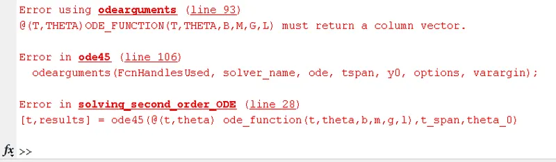
1. While defining the ode45 function, i had used comma instead of using a semicolon while defining `(d theta)/dt` and i obtained an error as it is supposed to be a column matrix.

Supposed to be :

Mistake :

Error Output :

The below error message was displayed in the command window as a result of the mistake.

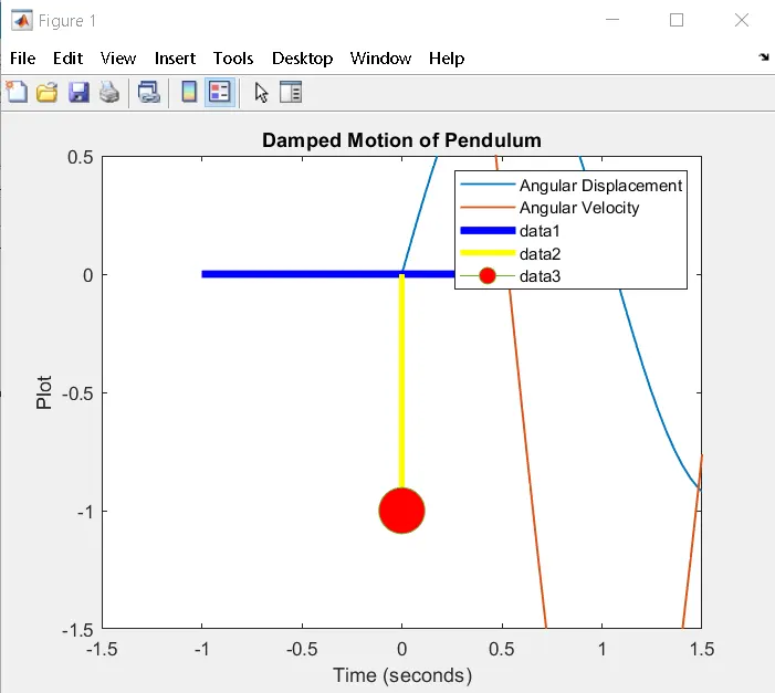
2. While plotting the second graph of animating the pendulum movement, i had forgotten to enter the "figure(2)" command in the program and i obtained a single mixed graph which was incorrect.

Supposed to be:

Mistake :

Output Result :

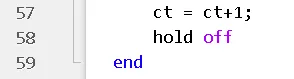
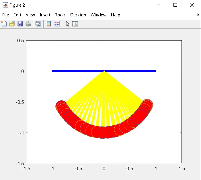
3. At the end off the program, i had not inserted the "hold off" command as a result of which, the entire path of the pendulum was traced on top of each other.

Supposed to be :

Mistake :

Output Result :

CONCLUSION :

1. The ODE representing a simple pendulum has been solved into two 1^st order equations as a function of time.

2. The graph showing the variation of angular displacement and angular velocity with change in time is obtained.

3. The animation movie simulating the Damped Harmonic Motion of a Simple Pendulum is obtained.