Project

Breaking Ice with Air cushion Vehicle - Finding minimum pressure with Newton-Raphson method using Python

NNikhil. S. Bharadwaj27 Mar 2023

AIM :

To write a Python program to calculate the minimum pressure required by air cushion vehicle to break ice of a certain thickness, using the Newton Raphson method.

OBJECTIVES :

Part-1 :
Calculate the values of cushion pressure (`p`) for the range of ice field thickness (`h`) = [ `0.6` , `1.2` , `1.8` , `2.4` , `3.0` , `3.6` , `4.2` ] by assuming a suitable relaxation factor.
Part-2 :
Use the Newton-Raphson method to find out the value of cushion pressure (`p`) for `h = 0.6` feet. Find the optimal relaxation factor for the same.

INTRODUCTION :

The Newton-Raphson method is a way to quickly find a good approximation for the root of a real-valued function `f(x) = 0`. It uses the idea that a continuous and differentiable function can be approximated by a straight line tangent to it.

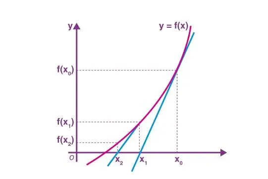
Suppose you need to find the root of a continuous, differentiable function `f(x)`, and you know the root you are looking for is near the point `x=x_0`. Then Newton's method tells us that a better approximation for the root is,

`x_1 = x_0 - (f(x_0))/(f'(x_0))`

This process may be repeated as many times as necessary to get the desired accuracy. In general, for any x-value (`x_n`), the next value is given by,

`x_(n+1) = x_n - (f(x_n))/(f'(x_n))`

Air Cushion Vehicle :

A conventional ACV uses mechanical advantage and the vessel’s mass to break ice downward in flexural stress. Then as the vessel progresses with its use of exceptional thrust, it rolls the ice pieces down, under, and to the side leaving a channel of reduced ice concentration in the vessels wake. For this method to work, ice must have somewhere to go and sufficiently deep water for the vessel to navigate.

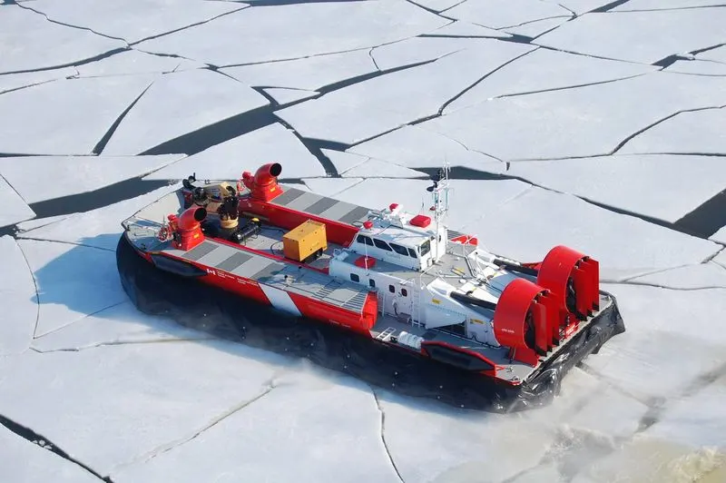
Dependent on ice thickness, a hovercraft can readily break ice in flexure by making a depression and send cracks through the ice. Once a crack is made, the path of least resistance for the hovercraft's air curtain gets under the ice and reduces the supporting water under the ice. The ice then fails under its own weight. At speed an ACV can setup a wave in the ice and send cracks through it.

This type of ice management is of value when ice is under horizontal stress say like an ice jam. What it does not do is clear or roll the ice out of the way. Shallow draft applications may take the form of ice management and attempts to clear river ice jams. Other applications include ice management without forcing ice into structures like inland harbours, piers, and boardwalks.

GOVERNING EQUATIONS :

The equation to calculate the cushion pressure required to break the ice field is given by.

`p^3(1-beta^2) + (0.4hbeta^2 – (sigmah^2)/r^2)p^2 + ((sigma^2h^4)/(3r^4))p – ((sigmah^2)/(3r^2))^3 = 0`

The derivative of the above function is given by.

`3p^2(1-beta^2) + 2p(0.4hbeta^2 – (sigmah^2)/r^2) + (sigma^2h^4)/(3r^4) = 0`

Where,

`p` = Cushion Pressure

`h` = Thickness of Ice Field

`r` = Size of Air Cushion

`sigma` = Tensile Strength of Ice

`beta` = Width of Ice Wedge

PART – 1 : CUSHION PRESSURE TO BREAK ICE

In this segment, we are going to calculate the cushion pressure required by the ACV to break ice of varying thickness, using the Newton-Raphson method.

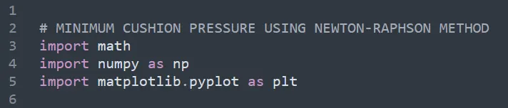
The first and foremost step is importing the necessary modules into Python. Here, we import the ‘numpy’, ‘matplotlib.pyplot’ and ‘math’ modules.

Inputs :

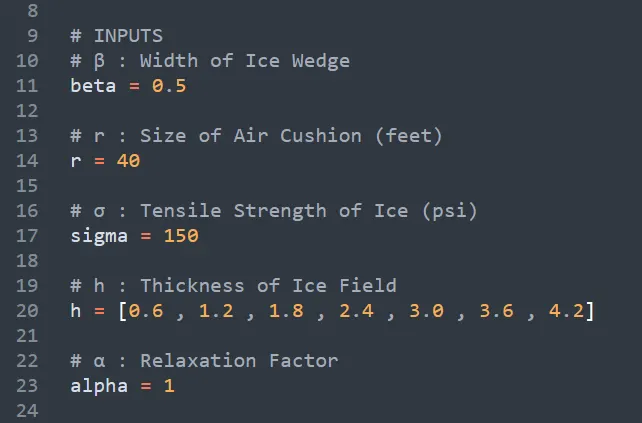
In this step, we define the various input parameters of the program.

Width of the Ice Wedge `beta = 0.5` `"feet"`
Size of Air Cushion `r = 40` `"feet"`
Tensile Strength of Ice `sigma = 150` `"psi"`
Thickness of Ice Field `h` = [ `0.6` , `1.2` , `1.8` , `2.4` , `3.0` , `3.6` , `4.2` ]
Relaxation Factor `alpha = 1`

User - Defined Functions :

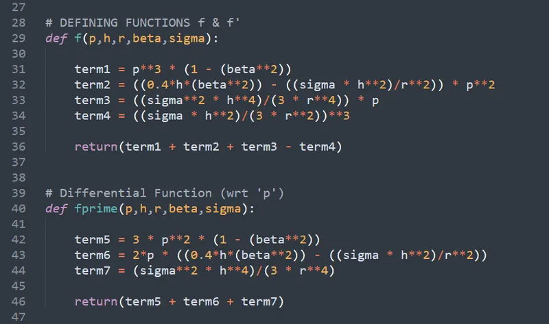
In this step, we define 2 functions representing the equations used to calculate the cushion pressure required to break the ice and the derivative of the equation.

The equation is divided into 4 parts for simplification and takes the inputs of ‘`h`’ , ‘`r`’ , ‘`sigma`’ and ‘`beta`’ to calculate the value of cushion pressure (`p`). The equation to calculate cushion pressure is given as,

`f(x) = p^3(1-beta^2) + (0.4hbeta^2 – (sigmah^2)/r^2)p^2 + ((sigma^2h^4)/(3r^4))p – ((sigmah^2)/(3r^2))^3`
Further, in order to solve the equations by using Newton-Raphson method, we find out the derivative of the above function. The derivative function is given as,

`f'(x) = 3p^2(1-beta^2) + 2p(0.4hbeta^2 – (sigmah^2)/r^2) + (sigma^2h^4)/(3r^4)`

Calculating Cushion Pressure & Number of Iterations :

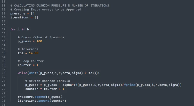
Here, we create empty arrays of pressure and iterations, which are going to be appended later on.
We use a ‘for loop’ for the range of values of ‘`h`’. We assume the initial guess value of pressure as `100` and a tolerance limit of `1e^(−06)`. We also define a loop counter, which at the end of the for loop, gives us the number of iterations run.
Inside the for loop, we define a ‘while loop’ condition such that values are within the tolerance limit. We include the Newton-Raphson formula inside the while loop and thereby, calculating our values of cushion pressure and the number of iterations run at the end of the loop. These values are then appended into the empty arrays.

Results :

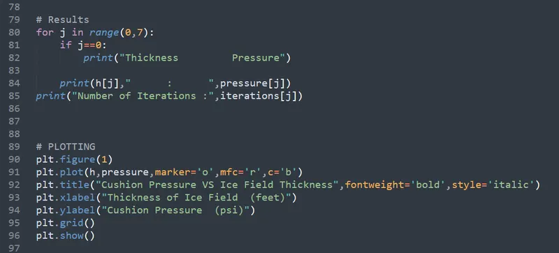
The calculated pressure values are displayed and the respective graphs are plotted as follows.

The values of cushion pressure calculated for different thicknesses of ice is displayed in the command window by using a ‘for loop’ command as shown.
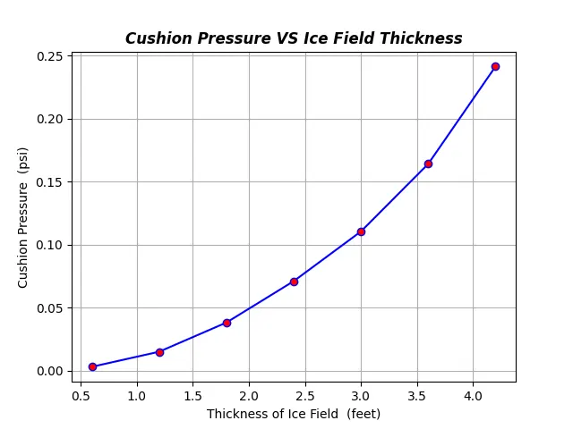
Finally, a graph representing “Cushion Pressure vs Ice Field Thickness” is plotted so as to observe the variation of required pressure with increase in ice thickness. The respective labels and title is provided as well.

OUTPUTS :

By running the above program code, we obtain our respective outputs as follows.

1. Pressure values for varying ice thickness.

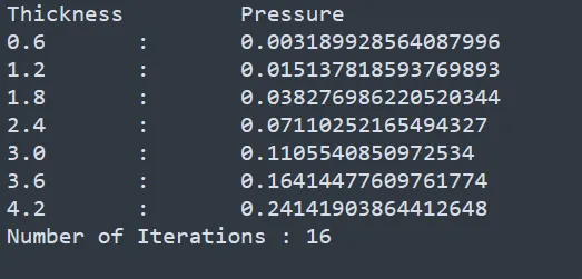
We can observe that with the increase in thickness of ice, the pressure required to break the ice also increases.

2. Plot of Cushion Pressure vs Ice Field Thickness

PART – 2 : OPTIMAL RELAXATION FACTOR

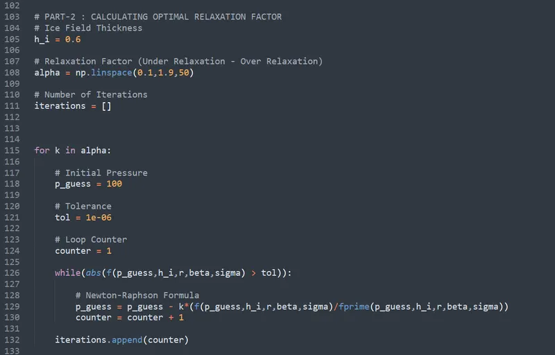
In the second section of the program, we write a python script to calculate the optimal relaxation factor such that the least number of iterations are run.

In order to do so, we first define an array representing the range of relaxation factors by using the ‘linspace’ command, out of which we find out the optimal relaxation factor. We maintain a constant ice field thickness of `0.6` feet.
Next, we define an empty array for the number of iterations, into which the value will be appended later on.
By assuming an initial guess value for pressure and a specific tolerance limit, we calculate the values of pressure and number of iterations run, by using the Newton-Raphson method. The number of iterations run are finally appended onto the empty array.

Results :

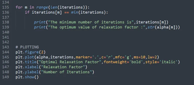
By using a ‘for loop’ for the range of values of number of iterations, we use a nested ‘if condition’ to calculate the value of minimum number of iterations run.
We use the ‘print’ commands to show the values of the minimum number of iterations and the corresponding relaxation factor value in the command window.
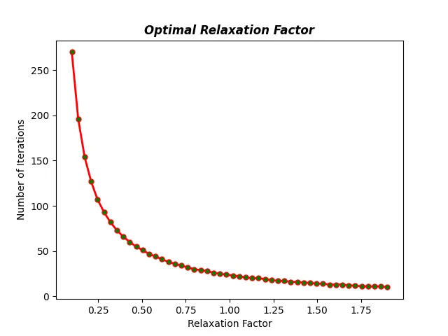
Finally, we plot a graph to observe the variation of number of iterations wrt to the relaxation factor values.

OUTPUTS :

By running the above program code, we obtain the following results.

1. Optimal Relaxation Factor Value

2. Relaxation Factor vs Number of Iterations

Final Program Code :

# MINIMUM CUSHION PRESSURE USING NEWTON-RAPHSON METHOD
import math
import numpy as np
import matplotlib.pyplot as plt



# INPUTS
# β : Width of Ice Wedge
beta = 0.5

# r : Size of Air Cushion (feet)
r = 40

# σ : Tensile Strength of Ice (psi)
sigma = 150

# h : Thickness of Ice Field
h = [0.6 , 1.2 , 1.8 , 2.4 , 3.0 , 3.6 , 4.2]

# α : Relaxation Factor
alpha = 1




# DEFINING FUNCTIONS f & f'
def f(p,h,r,beta,sigma):

	term1 = p**3 * (1 - (beta**2))
	term2 = ((0.4*h*(beta**2)) - ((sigma * h**2)/r**2)) * p**2
	term3 = ((sigma**2 * h**4)/(3 * r**4)) * p
	term4 = ((sigma * h**2)/(3 * r**2))**3

	return(term1 + term2 + term3 - term4)


# Differential Function (wrt 'p')
def fprime(p,h,r,beta,sigma):

	term5 = 3 * p**2 * (1 - (beta**2))
	term6 = 2*p * ((0.4*h*(beta**2)) - ((sigma * h**2)/r**2))
	term7 = (sigma**2 * h**4)/(3 * r**4)

	return(term5 + term6 + term7)




# CALCULATING CUSHION PRESSURE & NUMBER OF ITERATIONS
# Creating Empty Arrays to be Appended
pressure = []
iterations = []


for i in h:

	# Guess Value of Pressure
	p_guess = 100

	# Tolerance
	tol = 1e-06

	# Loop Counter
	counter = 1

	while(abs(f(p_guess,i,r,beta,sigma) > tol)):

		# Newton-Raphson Formula
		p_guess = p_guess - alpha*(f(p_guess,i,r,beta,sigma)/fprime(p_guess,i,r,beta,sigma))
		counter = counter + 1

	pressure.append(p_guess)
	iterations.append(counter)



# Results
for j in range(0,7):
	if j==0:
		print("Thickness         Pressure")

	print(h[j],"      :      ",pressure[j])
print("Number of Iterations :",iterations[j])



# PLOTTING
plt.figure(1)
plt.plot(h,pressure,marker='o',mfc='r',c='b')
plt.title("Cushion Pressure VS Ice Field Thickness",fontweight='bold',style='italic')
plt.xlabel("Thickness of Ice Field  (feet)")
plt.ylabel("Cushion Pressure  (psi)")
plt.grid()
plt.show()






# PART-2 : CALCULATING OPTIMAL RELAXATION FACTOR
# Ice Field Thickness
h_i = 0.6

# Relaxation Factor (Under Relaxation - Over Relaxation)
alpha = np.linspace(0.1,1.9,50)

# Number of Iterations
iterations = []



for k in alpha:

	# Initial Pressure
	p_guess = 100

	# Tolerance
	tol = 1e-06

	# Loop Counter
	counter = 1

	while(abs(f(p_guess,h_i,r,beta,sigma) > tol)):

		# Newton-Raphson Formula
		p_guess = p_guess - k*(f(p_guess,h_i,r,beta,sigma)/fprime(p_guess,h_i,r,beta,sigma))
		counter = counter + 1

	iterations.append(counter)


for m in range(len(iterations)):
	if iterations[m] == min(iterations):

		print("The minimum number of iterations is",iterations[m])
		print("The optimum value of relaxation factor :",str(alpha[m]))



# PLOTTING
plt.figure(2)
plt.plot(alpha,iterations,marker='.',c='r',mfc='g',ms=10,lw=2)
plt.title("Optimal Relaxation Factor",fontweight='bold',style='italic')
plt.xlabel("Relaxation Factor")
plt.ylabel("Number of Iterations")
plt.show()

CONCLUSIONS :

The python program to calculate the cushion pressure required to break the given thickness has been written and the outputs have been successfully obtained.

From the first plot, we can observe that with the increase in thickness of the ice, the pressure required to break it increases as well. Thereby, cushion pressure is directly proportional to ice thickness.

Finally, for a constant thickness of ice, the optimal relaxation factor value is found to be 1.9, which runs the least number of iterations, being 10.

Breaking Ice with Air cushion Vehicle - Finding minimum pressure with Newton-Raphson method using Python

Ship work like this
in your own course.

Talk to a career counsellor

Ship work like thisin your own course.

Talk to a career counsellor

Ship work like this
in your own course.