Week 3.5 - Deriving 4th order approximation of a 2nd order derivative using Taylor Table method
OBJECTIVES :
- To derive the fourth order approximation for the second order derivative using,
i.) Central Differencing Method
ii.) Skewed Right – Sided Differencing Method
iii.) Skewed Left – Sided Differencing Method - To write a program in Matlab to evaluate the second-order derivative of the analytical function `e^(x)*cos(x)` and compare it with the 3 numerical approximations that we have derived.
- Obtain a plot that compares the absolute error between all the three schemes.
INTRODUCTION :
In mathematics, the Taylor series of a function is an infinite sum of terms that are expressed in terms of the function's derivatives at a single point.
The Taylor series of a real or complex-valued function `f(x)`, is the power series,
`f(a) + (f'(a))/(1!)(x-a) + (f''(a))/(2!)(x-a)^2 + (f'''(a))/(3!)(x-a)^3 + ....`
In the more compact sigma notation, this can be written as,
`sum_(n=0)^oo f^n(a)/(n!) (x-a)^n`
Where, `f^(n)(a)` denotes the `n^(th)` derivative of `f` evaluated at the point `a`.
And `n!` denotes the factorial of `n`.
When a = 0, the series is also called a Maclaurin series.
FORMULAS AND CALCULATIONS :
Deriving the fourth order approximation for the second order derivative using,
- CENTRAL DIFFERENCING METHOD :
It is referred to as the Central Differencing Method because it takes the values from the current point as well as both the previous (L.H.S) and next (R.H.S) points.
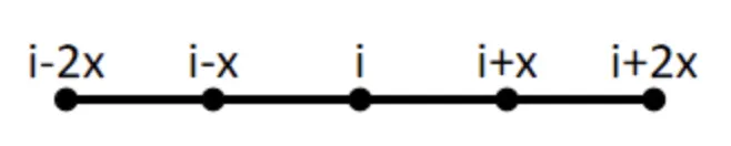
According to the given data, for a central differencing scheme,
Number of Nodes, N = P + Q - 1
Where,
P = Order of derivative
Q = Order of approximation.
As we are computing the 4th order approximation for a 2nd order derivative, we get
N = 2 + 4 – 1
Therefore, N = 5
This means that, we require 5 nodes to get the required accuracy.
Thereby, formulating the Hypothesis Equation, based on 5 nodes,
`(del^2u)/(delx^2) = (af(i-2) + bf(i-1) + cf(i) + df(i+1) + ef(i+2))/(Δx^2)` --- equation (1)
Taylor Series expansion terms :
➼ `af(i-2) = a[f(i) - (2Δx)f'(i) + (2Δx)^2/(2!)f''(i) - (2Δx)^3/(3!)f'''(i) + (2Δx)^4/(4!)f^(iv)(i) - (2Δx)^5/(5!)f^(v)(i)]`
➼ `bf(i-1) = b[f(i) - (Δx)f'(i) + (Δx)^2/(2!)f''(i) - (Δx)^3/(3!)f'''(i) + (Δx)^4/(4!)f^(iv)(i) - (Δx)^5/(5!)f^(v)(i)]`
➼ `cf(i) = cf(i)`
➼ `df(i+1) = d[f(i) + (Δx)f'(i) + (Δx)^2/(2!)f''(i) + (Δx)^3/(3!)f'''(i) + (Δx)^4/(4!)f^(iv)(i) + (Δx)^5/(5!)f^(v)(i)]`
➼ `ef(i+2) = e[f(i) + (2Δx)f'(i) + (2Δx)^2/(2!)f''(i) + (2Δx)^3/(3!)f'''(i) + (2Δx)^4/(4!)f^(iv)(i) + (2Δx)^5/(5!)f^(v)(i)]`
Taylor Table :
TAYLOR TABLE `Δx^2.(del^2u)/(delx^2)` Taylor Series Expansion Terms `f(i)` `(Δx)f'(i)` `(Δx)^2f''(i)` `(Δx)^3f'''(i)` `(Δx)^4f^(iv)(i)` `(Δx)^5f^(v)(i)` Numerical
Stencil
`af(i-2)` `a` `-2a` `2a` `-(8a)/6` `(16a)/24` `-(32a)/120` `bf(i-1)` `b` `-b` `b/2` `-b/6` `b/24` `-b/120` `cf(i)` `c` `0` `0` `0` `0` `0` `df(i+1)` `d` `d` `d/2` `d/6` `d/24` `d/120` `ef(i+2)` `e` `2e` `2e` `(8e)/6` `(16e)/24` `(32e)/120` `sum"co-efficients"` `0` `0` `1` `0` `0` `?`
Note :
- The sum of co-efficients of the second order derivative term (i.e, `Δx^2 f''(i)`) is 1, because we are trying to compute the second order derivative (`(del^2u)/(delx^2)`). Therefore, the only term that is supposed to be at the R.H.S is `f''(x)` term. Hence, we are equating it to 1.
- In the last column, which is the column of fifth order derivative term (`(Δx)^5f^(v)(i)`), we are representing a “`?`” sign for the sum of co-efficients. This is because, in our hypothesis equation, we have only 5 unknown terms (a , b , c , d and e). Therefore, for 5 unknowns we have 5 equations and if we add additional equations to it, we would be over specifying the system.
Equations :
➼ `a + b + c + d + e = 0`
➼ `-2a - b + 0 + d + 2e = 0`
➼ `2a + b/2 + 0 + d/2 + 2e = 1`
➼ `-(8a)/6 - b/6 + 0 + d/6 + (8e)/6 = 0`
➼ `(16a)/24 + b/24 + 0 + d/24 + (16e)/24 = 0`
Writing the above equations in matrix form to solve for the values for a , b , c , d and e.
`[[1,1,1,1,1],[-2,-1,0,1,2],[2,1/2,0,1/2,2],[-8/6,-1/6,0,1/6,8/6],[16/24,1/24,0,1/24,16/24]].[[a],[b],[c],[d],[e]] = [[0],[0],[1],[0],[0]]`
By solving the above matrix, we obtain the values,
`a = -1/12` , `b = 4/3` , `c = -5/2` , `d = 4/3` , `e = -1/12`
Thereby, substituting the above values in Hypothesis Equation - (1), we get
`Δx^2.(del^2u)/(delx^2) = -1/12.f(i-2) + 4/3.f(i-1) + -5/2.f(i) + 4/3.f(i+1) - 1/12f(i+2)`
Taking L.C.M of the denominator terms, we thereby obtain the Fourth Order Approximation Equation for Second Order Derivative by Central Differencing Method as follows,
`therefore` `(del^2u)/(delx^2) = (-f(x - 2Δx) + 16f(x - Δx) - 30f(x) + 16f(x + Δx) - f(x + 2Δx))/(12(Δx)^2)` - The sum of co-efficients of the second order derivative term (i.e, `Δx^2 f''(i)`) is 1, because we are trying to compute the second order derivative (`(del^2u)/(delx^2)`). Therefore, the only term that is supposed to be at the R.H.S is `f''(x)` term. Hence, we are equating it to 1.
-
SKEWED RIGHT – SIDED DIFFERENCING METHOD :
It is referred to as the Skewed Right - Sided Differencing Method because it takes the values from the current point as well as the next points (R.H.S).

According to the given data, for a skewed differencing scheme,
Number of Nodes, N = P + Q
Where,
P = Order of derivative
Q = Order of approximation.
As we are computing the 4th order approximation for a 2nd order derivative, we get
N = 2 + 4
Therefore, N = 6
This means that, we require 6 nodes to get the required accuracy.
Thereby, formulating the Hypothesis Equation, based on 6 nodes,
`Δx^2.(del^2u)/(delx^2) = af(i) + bf(i+1) + cf(i+2) + df(i+3) + ef(i+4) + gf(i+5)` --- equation (2)
Taylor Series expansion terms :
➼ `af(i) = af(i)`
➼ `bf(i+1) = b[f(i) + (Δx)f'(i) + (Δx)^2/(2!)f''(i) + (Δx)^3/(3!)f'''(i) + (Δx)^4/(4!)f^(iv)(i) + (Δx)^5/(5!)f^(v)(i)]`
➼ `cf(i+2) = c[f(i) + (2Δx)f'(i) + (2Δx)^2/(2!)f''(i) + (2Δx)^3/(3!)f'''(i) + (2Δx)^4/(4!)f^(iv)(i) + (2Δx)^5/(5!)f^(v)(i)]`
➼ `df(i+3) = d[f(i) + (3Δx)f'(i) + (3Δx)^2/(2!)f''(i) + (3Δx)^3/(3!)f'''(i) + (3Δx)^4/(4!)f^(iv)(i) + (3Δx)^5/(5!)f^(v)(i)]`
➼ `ef(i+4) = e[f(i) + (4Δx)f'(i) + (4Δx)^2/(2!)f''(i) + (4Δx)^3/(3!)f'''(i) + (4Δx)^4/(4!)f^(iv)(i) + (4Δx)^5/(5!)f^(v)(i)]`
➼ `gf(i+5) = g[f(i) + (5Δx)f'(i) + (5Δx)^2/(2!)f''(i) + (5Δx)^3/(3!)f'''(i) + (5Δx)^4/(4!)f^(iv)(i) + (5Δx)^5/(5!)f^(v)(i)]`
Taylor Table :
TAYLOR TABLE `Δx^2.(del^2u)/(delx^2)` Taylor Series Expansion Terms `f(i)` `(Δx)f'(i)` `(Δx)^2f''(i)` `(Δx)^3f'''(i)` `(Δx)^4f^(iv)(i)` `(Δx)^5f^(v)(i)` Numerical
Stencil
`af(i)` `a` `0` `0` `0` `0` `0` `bf(i+1)` `b` `b` `b/2` `b/6` `b/24` `b/120` `cf(i+2)` `c` `2c` `(4c)/2` `(8c)/6` `(16c)/24` `(32c)/120` `df(i+3)` `d` `3d` `(9d)/2` `(27d)/6` `(81d)/24` `(243d)/120` `ef(i+4)` `e` `4e` `(16e)/2` `(64e)/6` `(256e)/24` `(1024e)/120` `gf(i+5)` `g` `5g` `(25g)/2` `(125g)/6` `(625g)/24` `(3125g)/120` `sum"co-efficients"` `0` `0` `1` `0` `0` `0`
Equations :
➼ `a + b + c + d + e + g = 0`
➼ `0 + b + 2c + 3d + 4e + 5g = 0`
➼ `0 + b/2 + (4c)/2 + (9d)/2 + (16e)/2 + (25g)/2 = 1`
➼ `0 + b/6 + (8c)/6 + (27d)/6 + (64e)/6 + (125g)/6 = 0`
➼ `0 + b/24 + (16c)/24 + (81d)/24 + (256e)/24 + (625g)/24 = 0`
➼ `0 + b/120 + (32c)/120 + (243d)/120 + (1024e)/120 + (3125g)/120 = 0`
Writing the above equations in matrix form to solve for the values for a , b , c , d , e and g.
`[[1,1,1,1,1,1],[0,1,2,3,4,5],[0,1/2,2,9/2,8,25/2],[0,1/6,8/6,27/6,64/6,125/6],[0,1/24,16/24,81/24,256/24,625/24],[0,1/120,32/120,243/120,1024/120,3125/120]].[[a],[b],[c],[d],[e],[g]] = [[0],[0],[1],[0],[0],[0]]`
By solving the above matrix, we obtain the values,
`a = 15/4` , `b = -77/6` , `c = 107/6` , `d = -13` , `e = 61/12` , `g = -5/6`
Thereby, substituting the above values in Hypothesis Equation - (2), we get
`Δx^2.(del^2u)/(delx^2) = 15/4.f(i) - 77/6.f(i+1) + 107/6.f(i+2) - 13.f(i+3) + 61/12.f(i+4) - 5/6.f(i+5)`
Taking L.C.M of the denominator terms, we thereby obtain the Fourth Order Approximation Equation for Second Order Derivative by Skewed Right - Sided Differencing Method as follows,
`therefore` `(del^2u)/(delx^2) = (45f(x) - 154f(x + Δx) + 214f(x + 2Δx) - 156f(x + 3Δx) + 61f(x + 4Δx) - 10f(x + 5Δx))/(12(Δx)^2)` -
SKEWED LEFT – SIDED DIFFERENCING METHOD :
It is referred to as the Skewed Left - Sided Differencing Method because it takes the values from the current point as well as the previous points (L.H.S).

According to the given data, for a skewed differencing scheme,
Number of Nodes, N = P + Q
Where,
P = Order of derivative
Q = Order of approximation.
As we are computing the 4th order approximation for a 2nd order derivative, we get
N = 2 + 4
Therefore, N = 6
This means that, we require 6 nodes to get the required accuracy.
Thereby, formulating the Hypothesis Equation, based on 6 nodes,
`Δx^2.(del^2u)/(delx^2) = af(i) + bf(i-1) + cf(i-2) + df(i-3) + ef(i-4) + gf(i-5)` --- equation (3)
Taylor Series expansion terms :
➼ `af(i) = af(i)`
➼ `bf(i-1) = b[f(i) - (Δx)f'(i) + (Δx)^2/(2!)f''(i) - (Δx)^3/(3!)f'''(i) + (Δx)^4/(4!)f^(iv)(i) - (Δx)^5/(5!)f^(v)(i)]`
➼ `cf(i-2) = c[f(i) - (2Δx)f'(i) + (2Δx)^2/(2!)f''(i) - (2Δx)^3/(3!)f'''(i) + (2Δx)^4/(4!)f^(iv)(i) - (2Δx)^5/(5!)f^(v)(i)]`
➼ `df(i-3) = d[f(i) - (3Δx)f'(i) + (3Δx)^2/(2!)f''(i) - (3Δx)^3/(3!)f'''(i) + (3Δx)^4/(4!)f^(iv)(i) - (3Δx)^5/(5!)f^(v)(i)]`
➼ `ef(i-4) = e[f(i) - (4Δx)f'(i) + (4Δx)^2/(2!)f''(i) - (4Δx)^3/(3!)f'''(i) + (4Δx)^4/(4!)f^(iv)(i) - (4Δx)^5/(5!)f^(v)(i)]`
➼ `gf(i-5) = g[f(i) - (5Δx)f'(i) + (5Δx)^2/(2!)f''(i) - (5Δx)^3/(3!)f'''(i) + (5Δx)^4/(4!)f^(iv)(i) - (5Δx)^5/(5!)f^(v)(i)]`
Taylor Table :
TAYLOR TABLE `Δx^2.(del^2u)/(delx^2)` Taylor Series Expansion Terms `f(i)` `(Δx)f'(i)` `(Δx)^2f''(i)` `(Δx)^3f'''(i)` `(Δx)^4f^(iv)(i)` `(Δx)^5f^(v)(i)` Numerical
Stencil
`af(i)` `a` `0` `0` `0` `0` `0` `bf(i-1)` `b` `-b` `b/2` `-b/6` `b/24` `-b/120` `cf(i-2)` `c` `-2c` `(4c)/2` `-(8c)/6` `(16c)/24` `-(32c)/120` `df(i-3)` `d` `-3d` `(9d)/2` `-(27d)/6` `(81d)/24` `-(243d)/120` `ef(i-4)` `e` `-4e` `(16e)/2` `-(64e)/6` `(256e)/24` `-(1024e)/120` `gf(i-5)` `g` `-5g` `(25g)/2` `-(125g)/6` `(625g)/24` `-(3125g)/120` `sum"co-efficients"` `0` `0` `1` `0` `0` `0`
Equations :
➼ `a + b + c + d + e + g = 0`
➼ `0 - b - 2c - 3d - 4e - 5g = 0`
➼ `0 + b/2 + (4c)/2 + (9d)/2 + (16e)/2 + (25g)/2 = 1`
➼ `0 - b/6 - (8c)/6 - (27d)/6 - (64e)/6 - (125g)/6 = 0`
➼ `0 + b/24 + (16c)/24 + (81d)/24 + (256e)/24 + (625g)/24 = 0`
➼ `0 - b/120 - (32c)/120 - (243d)/120 - (1024e)/120 - (3125g)/120 = 0`
Writing the above equations in matrix form to solve for the values for a , b , c , d , e and g.
`[[1,1,1,1,1,1],[0,-1,-2,-3,-4,-5],[0,1/2,2,9/2,8,25/2],[0,-1/6,-8/6,-27/6,-64/6,-125/6],[0,1/24,16/24,81/24,256/24,625/24],[0,-1/120,-32/120,-243/120,-1024/120,-3125/120]].[[a],[b],[c],[d],[e],[g]] = [[0],[0],[1],[0],[0],[0]]`
By solving the above matrix, we obtain the values,
`a = -15/4` , `b = 77/6` , `c = -107/6` , `d = 13` , `e = -61/12` , `g = 5/6`
Thereby, substituting the above values in Hypothesis Equation - (3), we get
`Δx^2.(del^2u)/(delx^2) = -15/4.f(i) + 77/6.f(i+1) - 107/6.f(i+2) + 13.f(i+3) - 61/12.f(i+4) + 5/6.f(i+5)`
Taking L.C.M of the denominator terms, we thereby obtain the Fourth Order Approximation Equation for Second Order Derivative by Skewed Left - Sided Differencing Method as follows,
`therefore` `(del^2u)/(delx^2) = (-45f(x) + 154f(x + Δx) - 214f(x + 2Δx) + 156f(x + 3Δx) - 61f(x + 4Δx) + 10f(x + 5Δx))/(12(Δx)^2)`
PROGRAM AND EXPLANATION :
We are going to write a program to compare the absolute errors of the function `f(x) = e^x.cos(x)`, using the Central Difference, Skewed Right Sided Differencing and Skewed Left Sided Differencing methods.
Program :
% TAYLOR TABLE METHOD
clear all
close all
clc

% Inputs
x = pi/3;
dx = linspace(pi/4,pi/400,2000)


% ANALYTICAL DERIVATIVE
% Using uv rule for f(x)
% Double Differentiating as we require second order derivative
% f''(x) = -2*exp(x)*sin(x)
analytical_derivative = -2*exp(x)*sin(x)


% NUMERICAL DERIVATIVE
% CENTRAL DIFFERENCING METHOD
% Solving for co-efficients from matrix form
% In form of Ax = B
central_A = [[1,1,1,1,1];[-2,-1,0,1,2];[2,1/2,0,1/2,2];[-8/6,-1/6,0,1/6,8/6];[16/24,1/24,0,1/24,16/24]]
central_B = [0;0;1;0;0]
x_central = inv(central_A)*central_B


% SKEWED RIGHT - SIDED DIFFERENCING METHOD
% Solving for co-efficients from matrix form
% In form of Ax = B
skewed_right_A = [[1,1,1,1,1,1];[0,1,2,3,4,5];[0,1/2,2,9/2,8,25/2];[0,1/6,8/6,27/6,64/6,125/6];[0,1/24,16/24,81/24,256/24,625/24];[0,1/120,32/120,243/120,1024/120,3125/120]]
skewed_right_B = [0;0;1;0;0;0]
x_skewed_right = inv(skewed_right_A)*skewed_right_B


% SKEWED LEFT - SIDED DIFFERENCING METHOD
% Solving for co-efficients from matrix form
% In form of Ax = B
skewed_left_A = [[1,1,1,1,1,1];[0,-1,-2,-3,-4,-5];[0,1/2,2,9/2,8,25/2];[0,-1/6,-8/6,-27/6,-64/6,-125/6];[0,1/24,16/24,81/24,256/24,625/24];[0,-1/120,-32/120,-243/120,-1024/120,-3125/120]]
skewed_left_B = [0;0;1;0;0;0]
x_skewed_left = (skewed_left_A)^-1*skewed_left_B


% ANONYMOUS FUNCTION
f = @(x) exp(x).*cos(x)

% Difference Approximations
central_difference = ((x_central(1)*f(x-(2.*dx))) + (x_central(2)*f(x-dx)) + (x_central(3)*f(x)) + (x_central(4)*f(x+dx)) + (x_central(5)*f(x+(2.*dx))))./(dx.^2)
skewed_right_difference = ((x_skewed_right(1)*f(x)) + (x_skewed_right(2)*f(x+dx)) + (x_skewed_right(3)*f(x+(2.*dx))) + (x_skewed_right(4)*f(x+(3.*dx))) + (x_skewed_right(5)*f(x+(4.*dx))) + (x_skewed_right(6)*f(x+(5.*dx))))./(dx.^2)
skewed_left_difference = ((x_skewed_left(1)*f(x)) + (x_skewed_left(2)*f(x-dx)) + (x_skewed_left(3)*f(x-(2.*dx))) + (x_skewed_left(4)*f(x-(3.*dx))) + (x_skewed_left(5)*f(x-(4.*dx))) + (x_skewed_left(6)*f(x-(5.*dx))))./(dx.^2)


% COMPUTING ABSOLUTE ERROR
% error = numerical derivative - analytical derivative
central_differencing_error = abs(analytical_derivative - central_difference)
skewed_right_differencing_error = abs(analytical_derivative - skewed_right_difference)
skewed_left_differencing_error = abs(analytical_derivative - skewed_left_difference)


% PLOTTING ERROR GRAPH
loglog(dx,central_differencing_error,'LineWidth',1.5)
hold on
loglog(dx,skewed_right_differencing_error,'LineWidth',1.5)
loglog(dx,skewed_left_differencing_error,'LineWidth',1.5)
title('Taylor Table Method')
xlabel('dx')
ylabel('Absolute Error')
legend('Central Differencing','Skewed Right Sided Differencing','Skewed Left Sided Differencing')
Explanation :
- In the first and foremost step, we use the clear all, close all and clc commands to clear up the command window as well as the workspace.
- Next, for the given function `f(x)=e^(x)*cos(x)`, we define the input variable `x=π/3`.
Similarly, we define the range of dx by using the linspace command to obtain 2000 equally distributed values between `π/4` and `π/400`.
- To obtain the analytical derivative of the given function `f(x)`, we double differentiate the function using the uv rule and thereby we obtain the analytical derivative as `f''(x) = -2*e^(x)*sin(x)`. We are double differentiating the function as we require the second order derivative approximation.
- In the next steps, we calculate the unknown co-efficient values of the Hypothesis Equations for the Central, Skewed Right Sided and Skewed Left Sided Differencing Schemes. We do this by first formulating the equations from the respective Taylor Tables and then converting these equations into a matrix of the form `Ax + B`.
- After obtaining all the co-efficient values for the three schemes, we then define an Anonymous Function handle “ f ”. The @ operator creates the handle, and the parentheses ( ) immediately after the @ operator includes the function input arguments. This anonymous function accepts a single input x, and implicitly returns a single output, an array the same size as x that contains the function output value.
- Next, we calculate the absolute error between the analytical derivative and the obtained numerical derivative, by taking the difference between the two. We calculate the same for all the three schemes.
- Finally, we plot the log graphs of central, skewed right sided and skewed left sided approximation errors with respect to the range of dx. We complete the program by providing the respective titles, x & y labels and legends.
OUTPUT :
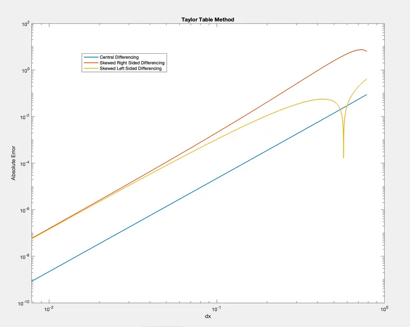
The above graph represents the variation in the errors of Central Differencing, Skewed Right Sided Differencing and Skewed Left Sided Differencing with respect to the range of dx.
CONCLUSION :
From the above plot, we can conclude that the error values of the Central Differencing Scheme are much lesser than those compared to the Skewed schemes. This is because the central differencing scheme takes values from both the left and right sides and thereby, the approximation is more accurate.
Why is a skewed scheme is useful? What can a skewed scheme do that a CD scheme cannot?
A skewed scheme is useful when we need to predict boundary conditions, because we need to calculate the values in only one direction. A central differencing scheme will not be useful in these kind of problems because it takes values from both the forward and backward directions.