Week 9 - FVM Literature Review
FINITE VOLUME METHOD (FVM) :
The finite volume method (FVM) is a discretization technique for partial differential equations, especially those that arise from physical conservation laws.
In the finite volume method, volume integrals in a partial differential equation that contain a divergence term are converted to surface integrals, using the divergence theorem. These terms are then evaluated as fluxes at the surfaces of each finite volume. Because the flux entering a given volume is identical to that leaving the adjacent volume, these methods are conservative. Another advantage of the finite volume method is that it is easily formulated to allow for unstructured meshes, therefore it is suitable for irregular and complex geometries.
The method is used in many computational fluid dynamics packages. "Finite volume" refers to the small volume surrounding each node point on a mesh.
FVM Methodology :
FVM is based on the integral form of the conservation laws, rather than their differential form. This leads to more accuracy/stability, especially for sharp gradients (i.e. large derivatives) inside a domain, which is also called shock-capturing property.
Furthermore, the FVM transforms the set of partial differential equations into a system of linear algebraic equations. Although the discrete approximation procedure in use in the FVM is distinctive, it also utilizes two basic steps.
- Firstly, it transforms and integrates the PDEs into balance equations over an element. The process incorporates the changing of the surface and volume integrals into discrete algebraic relations over elements as well as their surfaces using an integration quadrature of a specified order of accuracy. This will result in a set of semi-discrete equations.
- Secondly, in this next step, the interpolation profiles are chosen to estimate the variation of the variables within the element and relate the surface values of the variables to their cell values and thus transform the algebraic relations into algebraic equations. In regards to the two steps in the FVM process, your approximation selection affects the overall accuracy of the subsequent numeric.
Advantages and Disadvantages of FVM :
The FVM is a natural choice for solving CFD issues because the PDEs you have to resolve for CFD are conservation laws.
The FVM’s most significant advantage is that it only needs to do flux evaluation for the cell boundaries. Also, this is true for nonlinear issues as well, which, in turn, makes it an excellent choice for the handling of (nonlinear) conservation laws.
The accuracy of the FVM, for example, close to a corner of interest, can be increased by refining the mesh around that corner. However, the functions to estimate the solution is not easily made for higher-order. Therefore, this is a disadvantage of the FVM.
DIFFERENCES BETWEEN FDM AND FVM :
Similar to the finite difference method or finite element method, values are calculated at discrete places on a meshed geometry.
- In finite difference, the dependent variable values are stored at the nodes But in finite volume method, the dependent values are stored in the centre of the finite volume.
- In FVM, conservation of mass, momentum, energy is ensured at each cell/finite volume level. This is not true in finite difference and finite element approach.
- One advantage of the finite volume method over finite difference methods is that it does not require a structured mesh (although a structured mesh can also be used).
- FDM is a differential scheme, that is approximation of a taylor series expansion. We try to write the first order, second order differential in terms of difference between two point values. This may bring in some approximation error.
Finite Volume method is an integral scheme. Since you are integrating across the area, chance of error is minimized.
- Differential schemes are faster and error can be minimized if you have regular grids (squares and rectangles).
Integral schemes are slightly slower but score over FDM when the mesh is irregular.
Consider a 1-D steady state heat conduction equation which we are going to discretize using FVM.
`del/(delx)(alpha.(delT)/(delx)) + S = 0`
Where,
`S` = Source Term
`alpha` = Thermal Diffusivity (function of temperature and not a constant)
`(delT)/(delx)` = Temperature Gradient along x - direction
In FDM, we have nodal points over which we solve the equations. Whereas in FVM, the points are the centres of the volumes, which stores the average quantities inside the volume.
For 1-D, we have the volumes as follows,
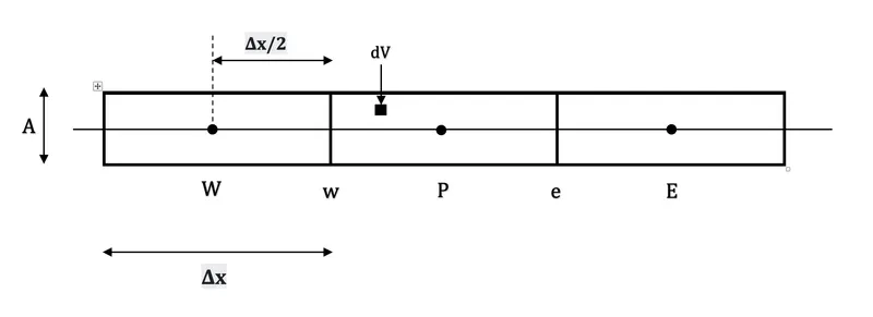
Considering control volume “P”, as shown in the above figure, surrounded by two control volumes E (east) and W (west) respectively. In our control volume, let us consider a very small volume “dV”. We solve our 1-D heat conduction equation in this volume dV and then we integrate it for the entire volume.
Therefore, the integral form of the governing equation is given by,
`int (del/(delx)(alpha.(delT)/(delx)) + S ).dV= 0`
Therefore, we are taking the conservation equation that is valid at a single point and we are saying that, if it is valid at a single point, it is valid at the entire volume and that the properties of the system are conserved.
`int^P del/(delx)(alpha.(delT)/(delx)).dV + intS .dV= 0`
From the figure, we know `dV = A.dx`
`int^P del/(delx)(alpha.(delT)/(delx)).A.dx + intS .dV= 0`
Integrating the above quantity, we get,
`[alphaA.(delT)/(delx)]_w^e + bar S .dV = 0`
Where, `barS` = average `S`, which when multiplied by `dV`, the entire control volume is going to be equal to that of integral "`S.dV`".
Therefore,
`alpha_eA. (delT)/(delx_e) - alpha_wA. (delT)/(delx_w) + barS.dV = 0`
Using approximations such as Taylor Series to calculate values of `(delT)/(delx)`,
`alphaA[(T_E - T_P)/(Deltax)] - alphaA[(T_P - T_W)/(Deltax)] + barS.dV = 0`
The above equation is in the form,
`"Heat Flux In" - "Heat Flux Out" + "Source Term" = 0` `->` Conserved Quantity
INTERPOLATION SCHEMES :
The evaluation of surface and volume integrals in our finite volume formulation require the value of the unknown variables at locations other than the computational nodes of the control volume. So, we need some sort of mathematical approximation or schemes to compute the values at these locations, and that is why we need various types of interpolation schemes.
There are numerous interpolation schemes such as,
- Upwind Interpolation Scheme (UDS) :
Upwind interpolation scheme is essentially used for convection dominated problems. The name upwind signifies that we are going to make use of the node which is upwind or upstream of the given node.
The use of upwind interpolation scheme is equivalent to using a backward or forward finite difference approximation, depending on the flow direction.
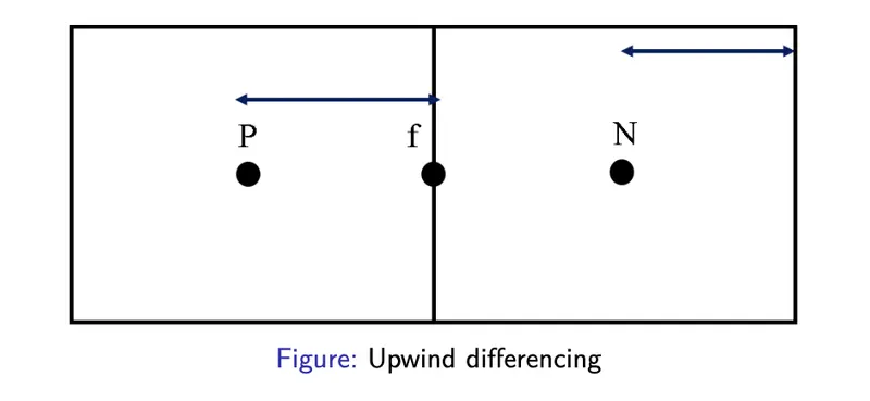
The use of upwind interpolation leads to a scheme which is first order accurate, as is not linearly varying. Hence, very fine grids are required to obtain accurate results.
The advantage of this scheme is that, it is the only approximation that satisfies boundedness criterion unconditionally. In the sense, irrespective of what the velocity values are and irrespective of what the grid spacing is, the solution will always remain bounded. Therefore, the use of upwind interpolation will never yield oscillatory solutions.
- Linear Interpolation (CDS) :
In linear interpolation scheme, which is termed in short as CDS (Central Differencing Scheme), we approximate the value of a variable at the control volume face centre by linear interpolation of the values at the two nearest computational nodes. This linear interpolation is equivalent to the use of central difference formula of the first order derivative. Hence, this scheme is also termed as central difference scheme or CDS.
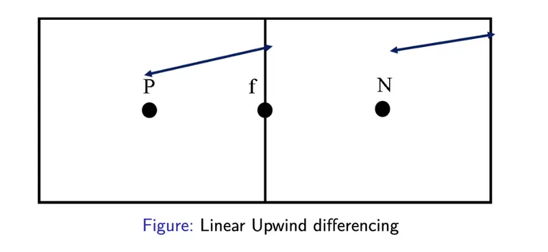
The characteristics of the CDS is that it is second order accurate, but for advection dominated situations, this scheme may produce oscillatory solutions (if the grid spacing is very large). On the positive side, it is the simplest and the most widely used interpolation scheme. It is used very commonly, especially in flow simulations which require the use of finite spatial and temporal grids.
- Quadratic Upwind Interpolation (QUICK) :
This scheme was derived by Leonard in 1979 and he named this scheme as QUICK, which is basically an acronym that stands for Quadratic Upwind Interpolation for Convective Kinematics. Convective kinematics because this particular interpolation would be used for convection dominated problems and quadratic because we have obtained this interpolation based on quadratic interpolation formulae.
One of the main objectives of this scheme was that we can get a second order accurate scheme, which has better damping properties than CDS and better accuracy than UDS. So, the quick upwind interpolation schemes was devised for this particular purpose. The name upwind, tells us we are going to get more prominence or more weightage to the function values at the nodes which are on the upstream side.
This particular scheme it is third order accurate in both uniform and non-uniform grids.
- Hybrid Interpolation Scheme :
Hybrid Interpolation Scheme is a blend of CDS and UDS, based on the local peclet number. The hybrid interpolation scheme combines the desirable properties of both CDS and UDS.
Some of the other interpolation schemes that are used are TVD, which stands for Total Variation Dimensions schemes and also ENO, which stands for Essentially Non-Oscillatory interpolation schemes.
FLUX LIMITERS :
Flux limiters are used in high resolution schemes – numerical schemes used to solve problems in science and engineering, particularly fluid dynamics, described by partial differential equations (PDEs). They are used to avoid the spurious oscillations (wiggles) that would otherwise occur with high order spatial discretization schemes due to shocks, discontinuities or sharp changes in the solution domain. Use of flux limiters, together with an appropriate high resolution scheme, make the solutions total variation diminishing (TVD).
The main idea behind the construction of flux limiter schemes is to limit the spatial derivatives to realistic values – for scientific and engineering problems this usually means physically realisable and meaningful values.
Flux limiters are also referred to as slope limiters because they both have the same mathematical form, and both have the effect of limiting the solution gradient near shocks or discontinuities. In general, the term flux limiter is used when the limiter acts on system fluxes, and slope limiter is used when the limiter acts on system states (like pressure, velocity etc).
The limiter function is constrained to be greater than or equal to zero, i.e., `phi(r)>= 0`. Therefore, when the limiter is equal to zero (sharp gradient, opposite slopes or zero gradient), the flux is represented by a low resolution scheme. Similarly, when the limiter is equal to 1 (smooth solution), it is represented by a high resolution scheme. The various limiters have differing switching characteristics and are selected according to the particular problem and solution scheme. No particular limiter has been found to work well for all problems, and a particular choice is usually made on a trial and error basis.