Week 6 - CHT Analysis on a Graphics card

AIM:

• To perform Steady State Conjugate Heat Transfer analysis on a Graphics Card.

OBJECTIVE:

• To perform the simulation with a baseline mesh and then refine it with the best possible element size.
• Properly defining the fluid and solid zones and using appropriate solid materials for different components.
• To perform the simulation for three different cases and compare the results.
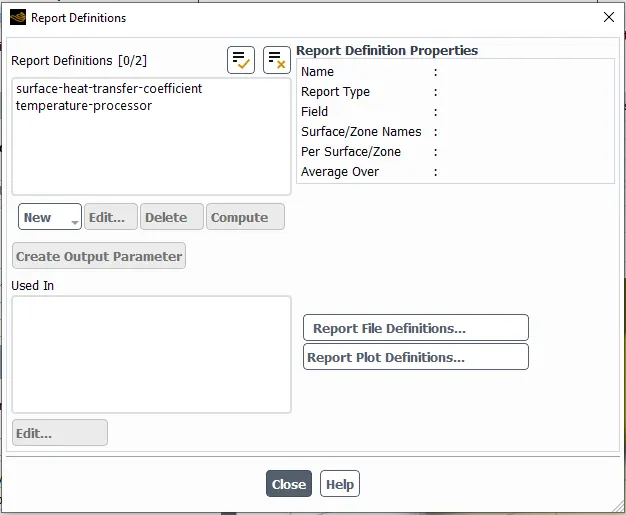
• To calculate the Heat transfer Coefficient and the Maximum Temperature achieved by the Processor.
• To show the simulation has achieved convergence with appropriate plots and images.
• To identify the hotspot regions of the Graphics Card.

INTRODUCTION:

CONJUGATE HEAT TRANSFER ANALYSIS:

• The Conjugate Heat Transfer (CHT) analysis type allows for the simulation of heat transfer between solid and fluid domains by exchanging thermal energy at the interfaces between them. Typical applications of this analysis type exist as, but are not limited to, the simulation of heat exchangers, cooling of electronic equipment, and general-purpose cooling and heating systems. Efficiently combining heat transfer in fluids and solids is the key to designing effective coolers, heaters, or heat exchangers.

• The fluid usually plays the role of energy carrier on large distances. Forced convection is the most common way to achieve high heat transfer rate. In some applications, the performances are further improved by combining convection with phase change (for example liquid water to vapour phase change). Even so, solids are also needed, in particular to separate fluids in a heat exchanger so that fluids exchange energy without being mixed.

• The temperature field and the heat flux are continuous at the fluid/solid interface. However, the temperature field can rapidly vary in a fluid in motion: close to the solid, the fluid temperature is close to the solid temperature, and far from the interface, the fluid temperature is close to the inlet or ambient fluid temperature. The distance where the fluid temperature varies from the solid temperature to the fluid bulk temperature is called the thermal boundary layer. The thermal boundary layer size and the momentum boundary layer relative size is reflected by the Prandtl number. For the Prandtl number to equal 1, thermal and momentum boundary layer thicknesses need to be the same. A thicker momentum layer would result in a Prandtl number larger than 1. Conversely, a Prandtl number smaller than 1 would indicate that the momentum boundary layer is thinner than the thermal boundary layer. The Prandtl number for air at atmospheric pressure and at 20°C is 0.7. That is because for air, the momentum and thermal boundary layer have similar size, while the momentum boundary layer is slightly thinner than the thermal boundary layer. For water at 20°C, the Prandtl number is about 7. So, in water, the temperature changes close to a wall are sharper than the velocity change.

  Heat transfer in solids and heat transfer in fluids are combined in the majority of applications. This is because fluids flow around solids or between solid walls, and because solids are usually immersed in a fluid. An accurate description of heat transfer modes, material properties, flow regimes, and geometrical configurations enables the analysis of temperature fields and heat transfer. Such a description is also the starting point for a numerical simulation that can be used to predict conjugate heat transfer effects or to test different configurations in order, for example, to improve thermal performances of a given application.

APPLICATIONS:

• Computational Fluid Dynamics (CFD) and more specifically conjugate heat transfer (CHT) analysis can accurately predict heat transfer by simultaneous solving all the relevant solid and flow field heat transfer processes, for example: conduction through solids, free and forced convection in the gases/fluids and thermal radiation.

• The CHT approach has an advantage over FE thermal analysis in that wall heat transfer coefficients and their local variations on surfaces are directly calculated within the model rather than based on simplified empirical calculations. The CHT approach therefore has benefits for those applications where heat transfer is either non-uniform or difficult to calculate empirically.

• The heat transfer projects have covered a wide range of aerodynamic and hydrodynamic industrial applications but projects typically had objectives such as:

  1. Temperature distribution analysis.
  2. Heat flux rate analysis – calculation of wall heat flux rates or heat transfer coefficients.
  3. Visualization of heat transfer features for improved understanding of system flow phenomena.
  4. Identification of localized ‘hot spots or heat sinks in checking against specified requirements.
  5. Evaluating variation in temperature peaks for different operating conditions/ failure modes.
  6. Assessing insulation or heat shield effectiveness and optimizing of material selections.
  7. Coupling CHT with FE analysis to evaluate thermally induced stresses, expansion or fatigue.
  8. Temperature field analysis
  9. CFD thermal analysis
  10. Heat transfer coefficient analysis
  11. Heat transfer rate analysis

METHODOLOGY:

• The graphics card present inside a computer generates heat depending upon the load of the computer.
• Practically the graphics card uses 100 W to 300 W of energy depending upon the load given to it and generates heat.
• This heat is dissipated to the surrounding components and in order to prevent damage of different electronic components and prevent fire we need to cool down the Processor.
• So, Heat Sink with multiple fins are present above the processor which conducts the heat from the processor and cools it down by the air.
• Multiple fins are present to increase the surface area so that the air coming have maximum area of contact and the processor cools down faster.
• Here both conduction in the components and convection due to the air takes place.
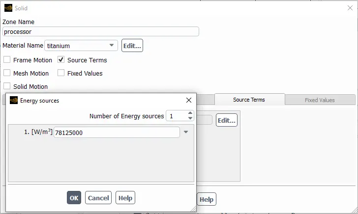
• So, in order to simulate the above we need to define the heat generation source term for the processor.
• To do so first we need to calculate the volume of the processor.
• The area of the processor is 32e-06 m^2.
• The volume of the processor is 64e-09 m^3.
• Since this is a very small replica of the actual graphics card we will assume a wattage of 5 Watts used by the processor.
• Heat Generated = `5/(64 X 10^-9)` W/m^3
  • = 78125000 W/m^3

CASE - 1:

• Baseline Mesh
• Mesh Element Size: 10.289 mm
• Total Elements: 83285
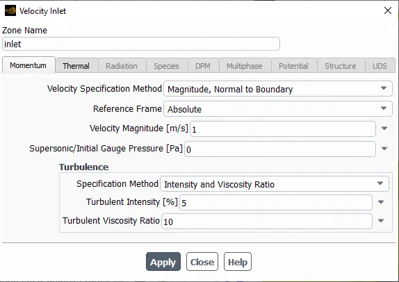
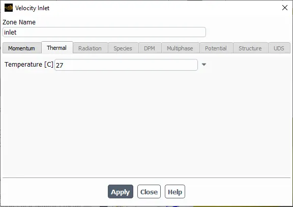
• Inlet Velocity: 1m/s

GEOMETRY:

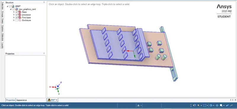
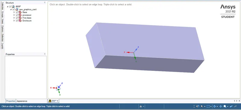
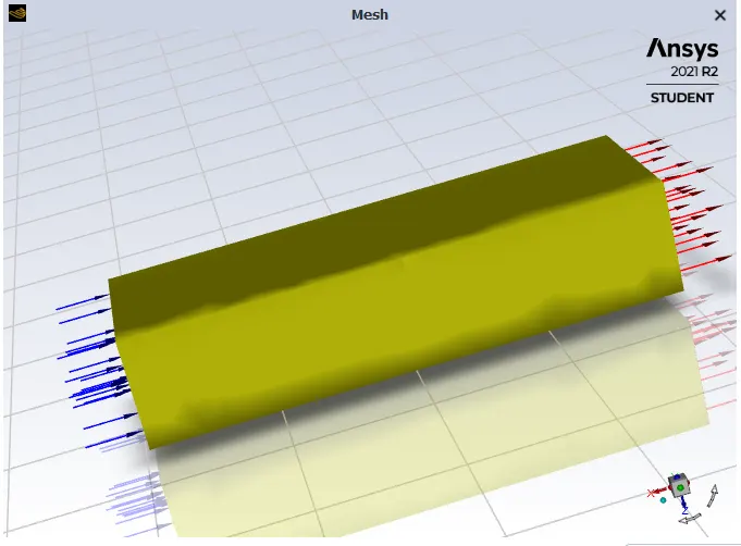
• In Ansys Spaceclaim we need to enable the share in the topology box and perform the share operation from the workbench menu so that all the walls of the component share their common boundary and we will get a conformal mesh.

MESHING:

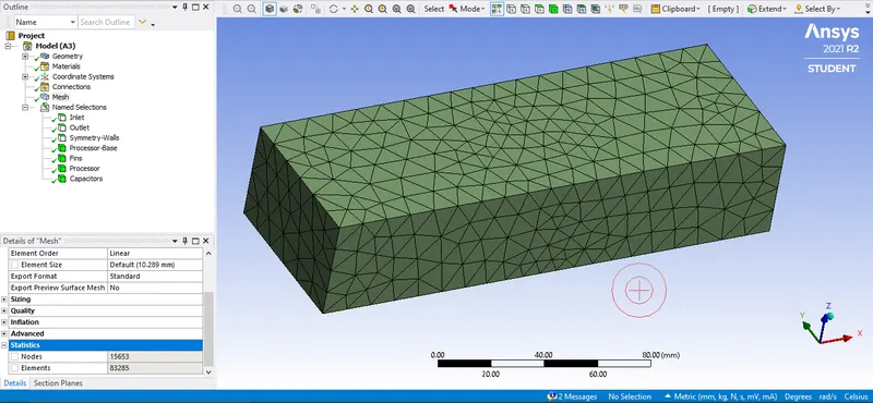
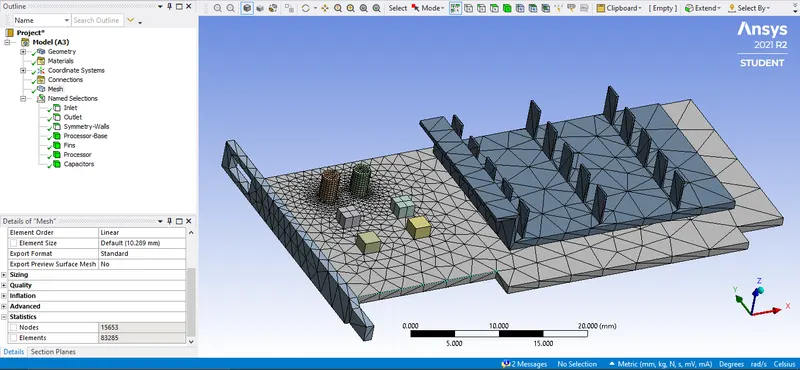
• Here in meshing we need to properly name the components and faces as per required and check that after generation of mesh it generates conformal mesh.
• It's very important to have conformal mesh in this assignment so that the heat generated from the processor travels properly to the neighboring components so that the heat generated from it gets dissipated and we get the correct result from the simulation.

SETUP:

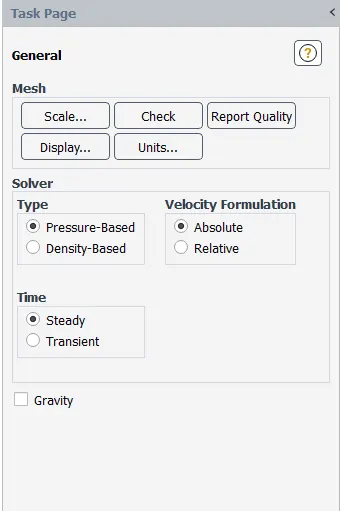
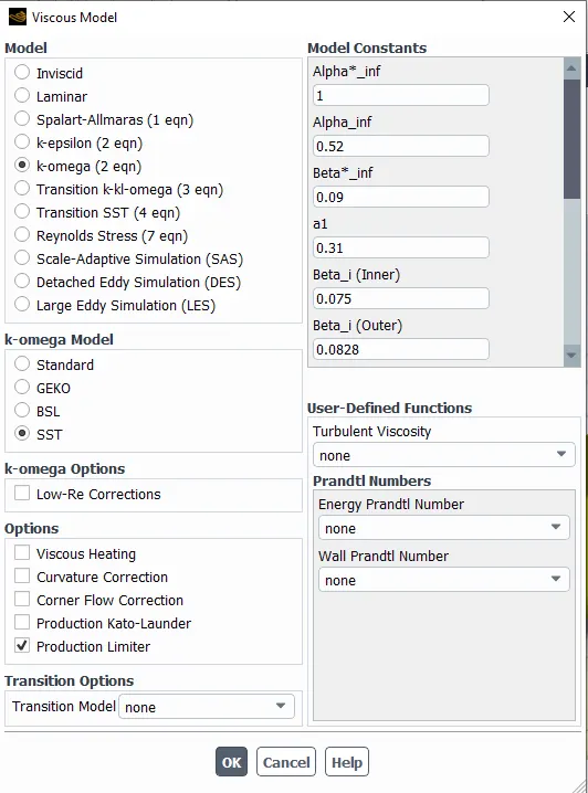
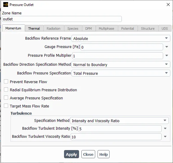
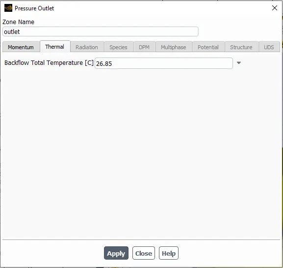
• In this assignment we are using the K-Omega SST turbulence model to run the simulation.
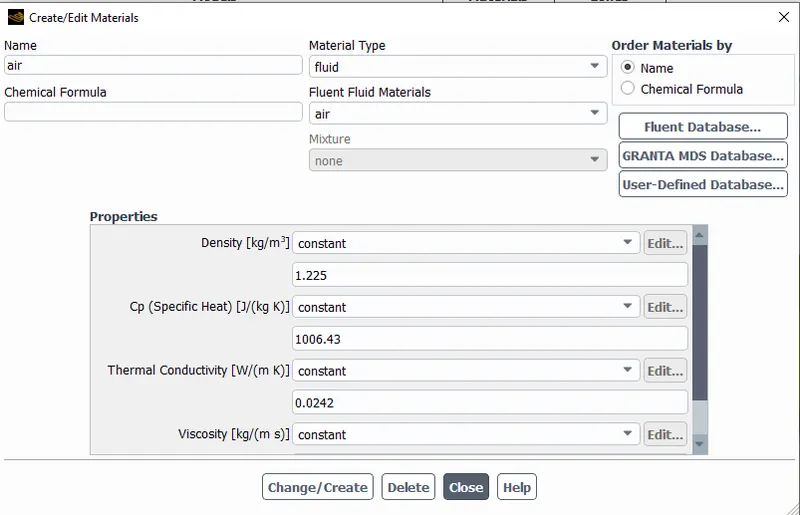
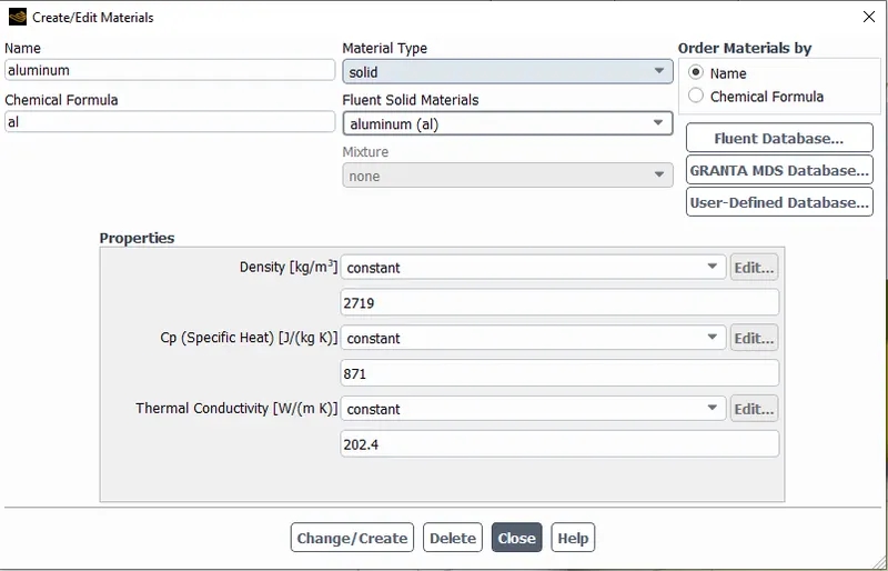
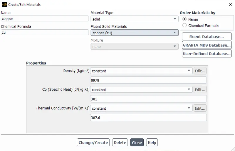
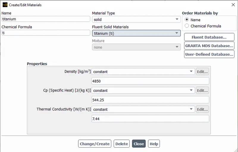
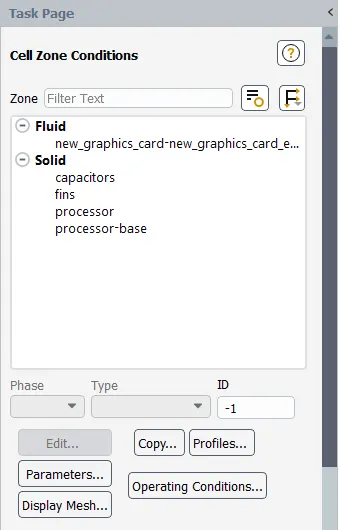
• We have to select proper material for different components of the graphics card.
• Processor: Titanium
• Base: Copper
• Heat Sink: Aluminum
• We have to define the heat generation source term for the processor that is 78125000 W/m^3.

RESULTS:

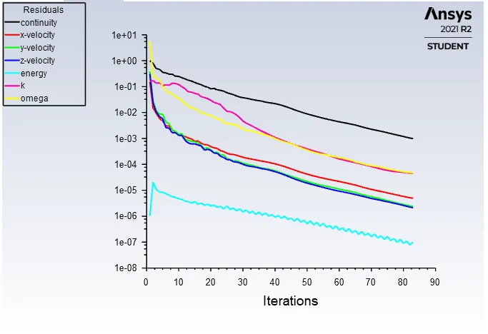
RESIDUALS:

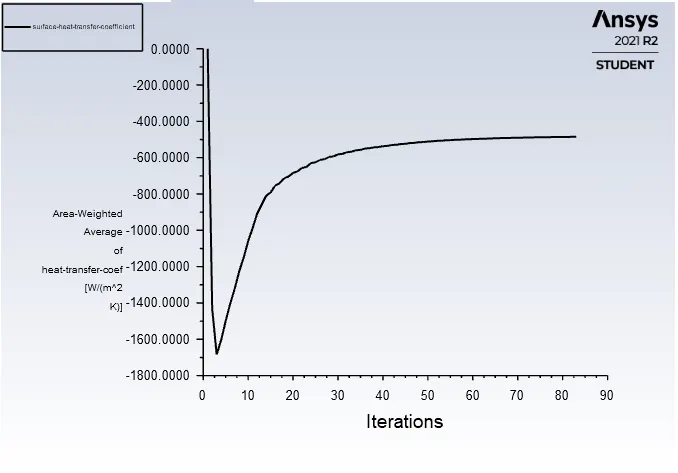
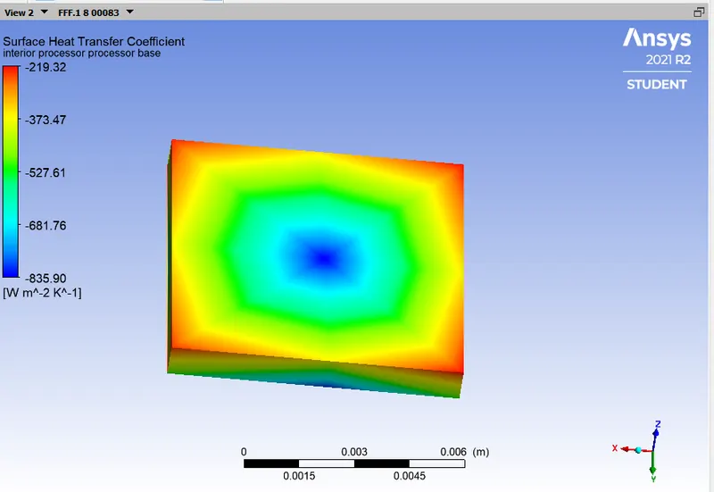
HEAT TRANSFER COEFFICIENT OF PROCESSOR:

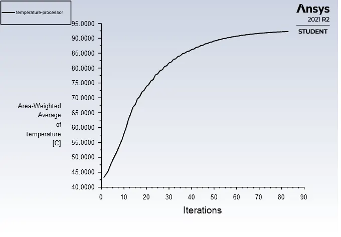
MAXIMUM TEMPERATURE OF PROCESSOR:

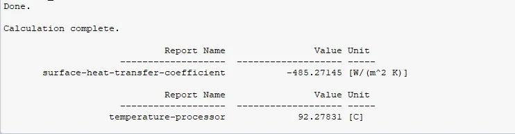
VALUES:

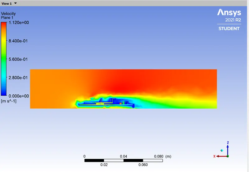
VELOCITY CONTOUR:

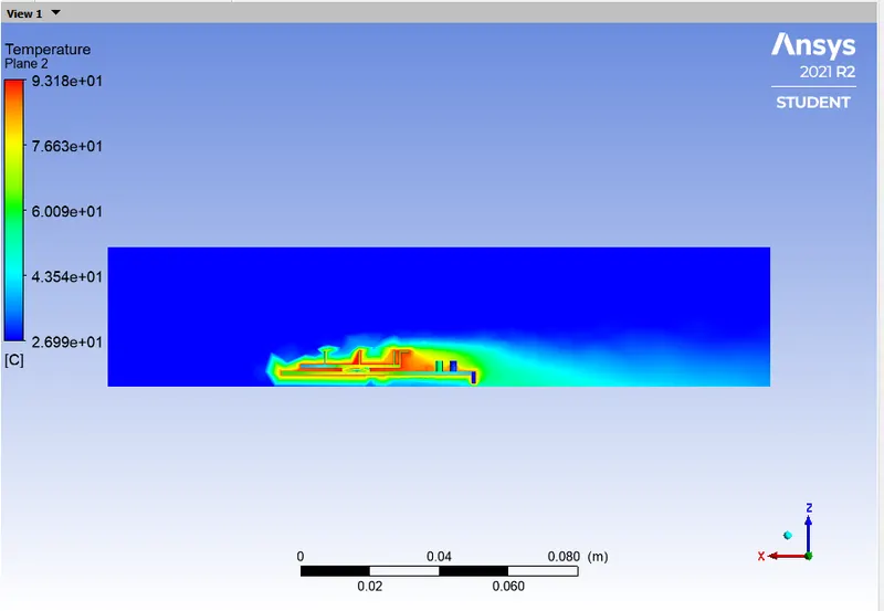
TEMPERATURE CONTOUR:

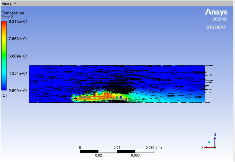
TEMPERATURE CONTOUR WITH VELOCITY VECTORS:

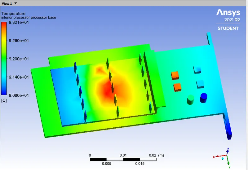
TEMPERATURE CONTOUR ON THE GRAPHICS CARD:

TEMPERATURE CONTOUR ON THE PROCESSOR:

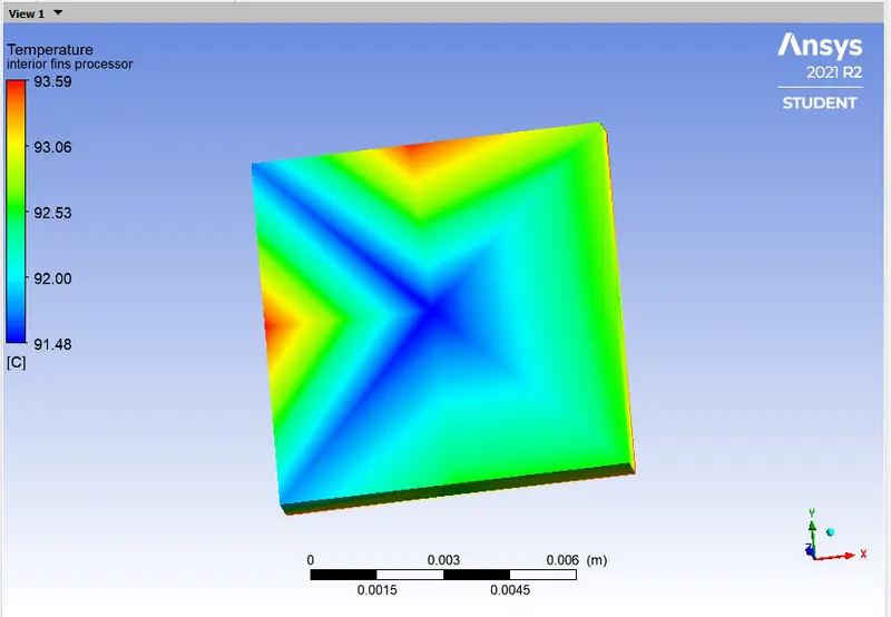
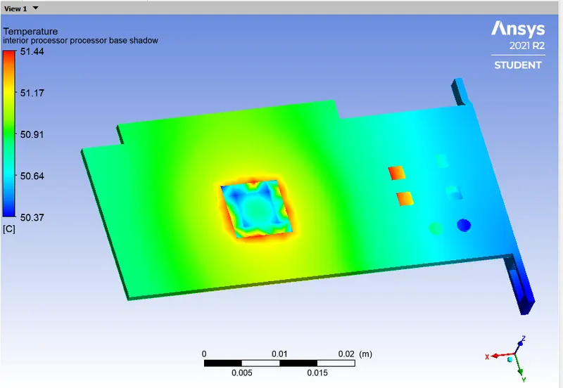
TEMPERATURE CONTOUR ON THE BASE:

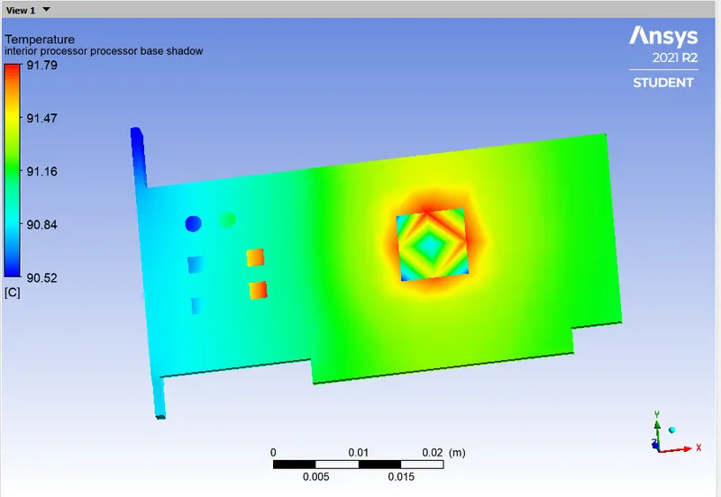
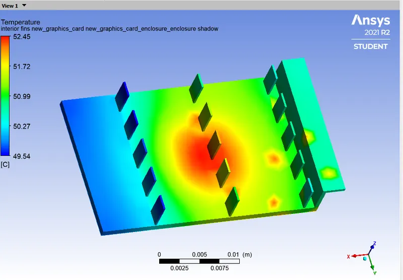
TEMPERATURE CONTOUR ON THE HEAT SINK:

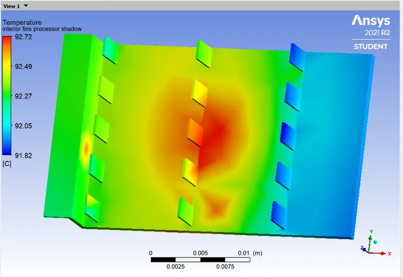
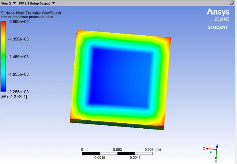
TEMPERATURE CONTOUR OF SURFACE HEAT TRANSFER COEFFICIENT OF THE PROCESSOR:

CASE - 2:

• Refined Mesh
• Mesh Element Size: 1.6 mm
• Total Elements: 499615
• Inlet Velocity: 1m/s

GEOMETRY:

• In Ansys Spaceclaim we need to enable the share in the topology box and perform the share operation from the workbench menu so that all the walls of the component share their common boundary and we will get a conformal mesh.

MESHING:

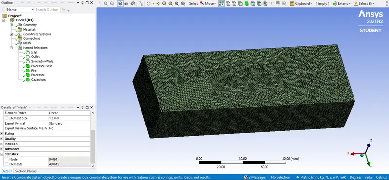
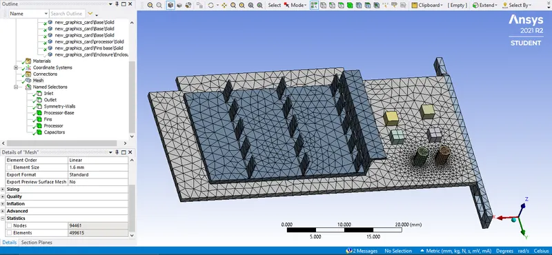
• As per trial error method we got the Mesh element size as 1.6mm as the best possible size as the total number of elements are 499615 which can be simulated without any problem.
• Here in meshing we need to properly name the components and faces as per required and check that after generation of mesh it generates conformal mesh.
• It's very important to have conformal mesh in this assignment so that the heat generated from the processor travels properly to the neighboring components so that the heat generated from it gets dissipated and we get the correct result from the simulation.

SETUP:

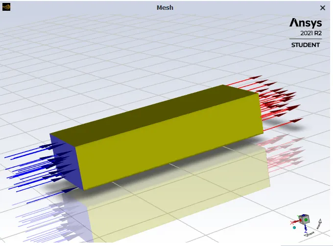
• In this assignment we are using the K-Omega SST turbulence model to run the simulation.
• We have to select proper material for different components of the graphics card.
• Processor: Titanium
• Base: Copper
• Heat Sink: Aluminum
• We have to define the heat generation source term for the processor that is 78125000 W/m^3.

RESULTS:

RESIDUALS:

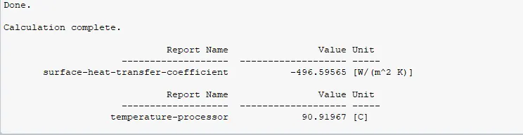
HEAT TRANSFER COEFFICIENT OF PROCESSOR:

MAXIMUM TEMPERATURE OF PROCESSOR:

VALUES:

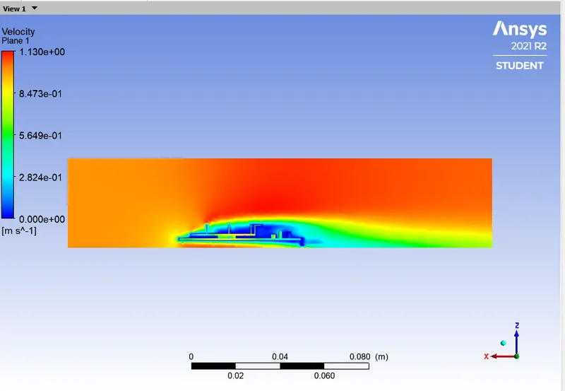
VELOCITY CONTOUR:

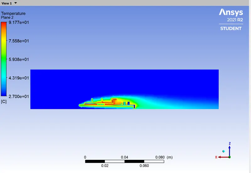
TEMPERATURE CONTOUR:

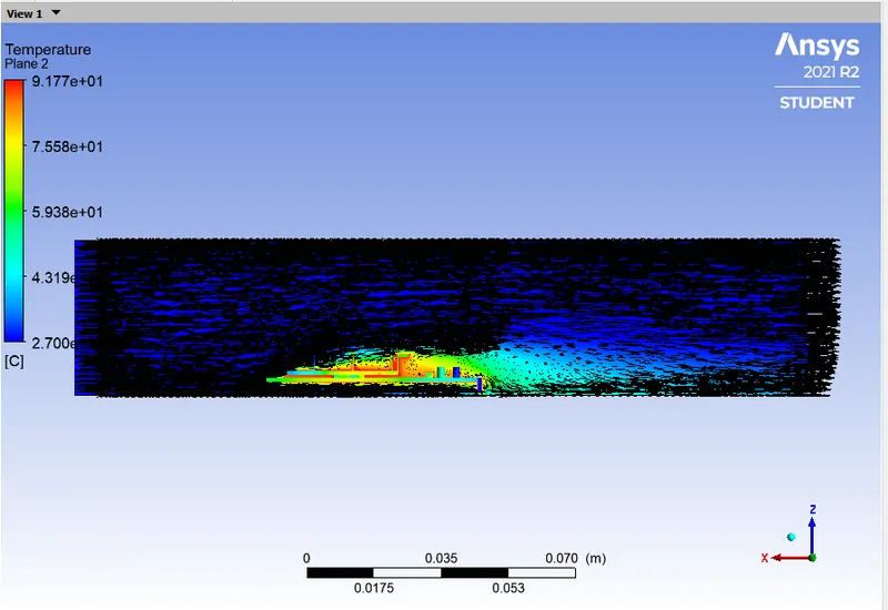
TEMPERATURE CONTOUR WITH VELOCITY VECTORS:

TEMPERATURE CONTOUR ON THE GRAPHICS CARD:

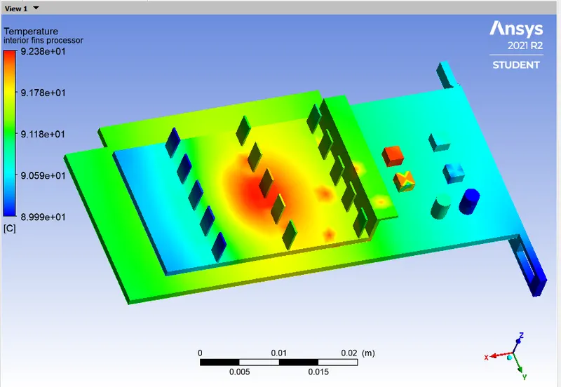
TEMPERATURE CONTOUR ON THE PROCESSOR:

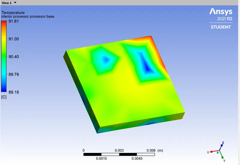
TEMPERATURE CONTOUR ON THE BASE:

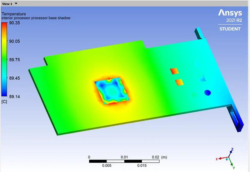
TEMPERATURE CONTOUR ON THE HEAT SINK:

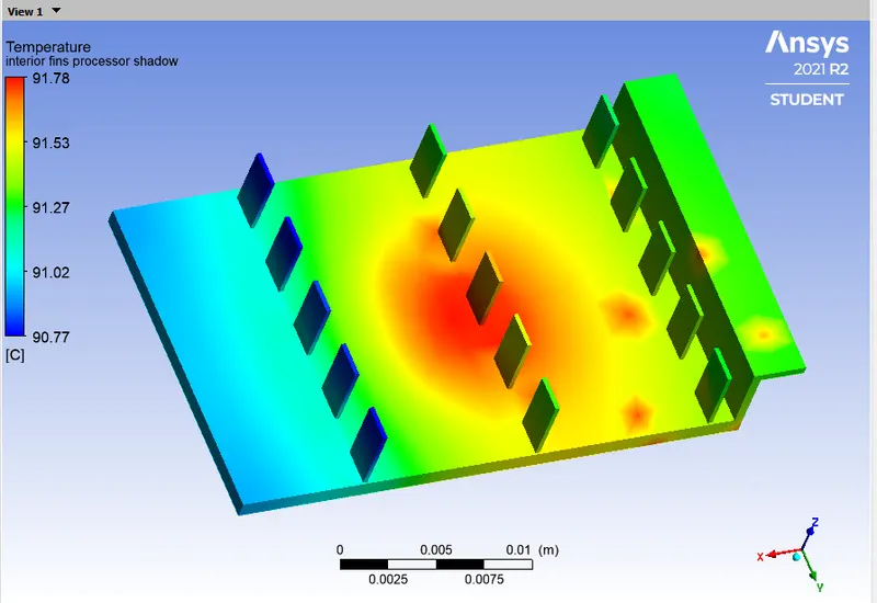
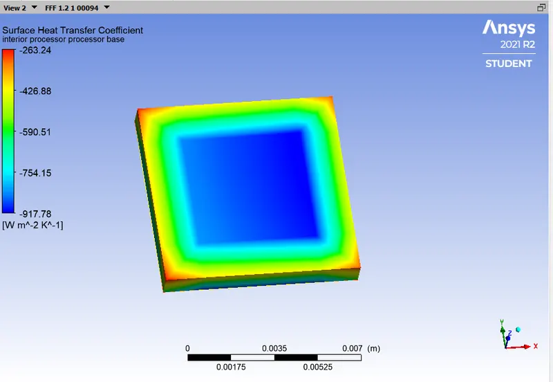
TEMPERATURE CONTOUR OF SURFACE HEAT TRANSFER COEFFICIENT OF THE PROCESSOR:

CASE - 3:

• Refined Mesh
• Mesh Element Size: 1.6 mm
• Total Elements: 499615
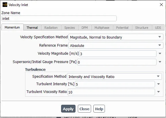
• Inlet Velocity: 3m/s

GEOMETRY:

• In Ansys Spaceclaim we need to enable the share in the topology box and perform the share operation from the workbench menu so that all the walls of the component share their common boundary and we will get a conformal mesh.

MESHING:

• As per trial error method we got the Mesh element size as 1.6mm as the best possible size as the total number of elements are 499615 which can be simulated without any problem.
• Here in meshing we need to properly name the components and faces as per required and check that after generation of mesh it generates conformal mesh.
• It's very important to have conformal mesh in this assignment so that the heat generated from the processor travels properly to the neighboring components so that the heat generated from it gets dissipated and we get the correct result from the simulation.

SETUP:

• In this assignment we are using the K-Omega SST turbulence model to run the simulation.
• We have to select proper material for different components of the graphics card.
• Processor: Titanium
• Base: Copper
• Heat Sink: Aluminum
• We have to define the heat generation source term for the processor that is 78125000 W/m^3.

RESULTS:

RESIDUALS:

HEAT TRANSFER COEFFICIENT OF PROCESSOR:

MAXIMUM TEMPERATURE OF PROCESSOR:

VALUES:

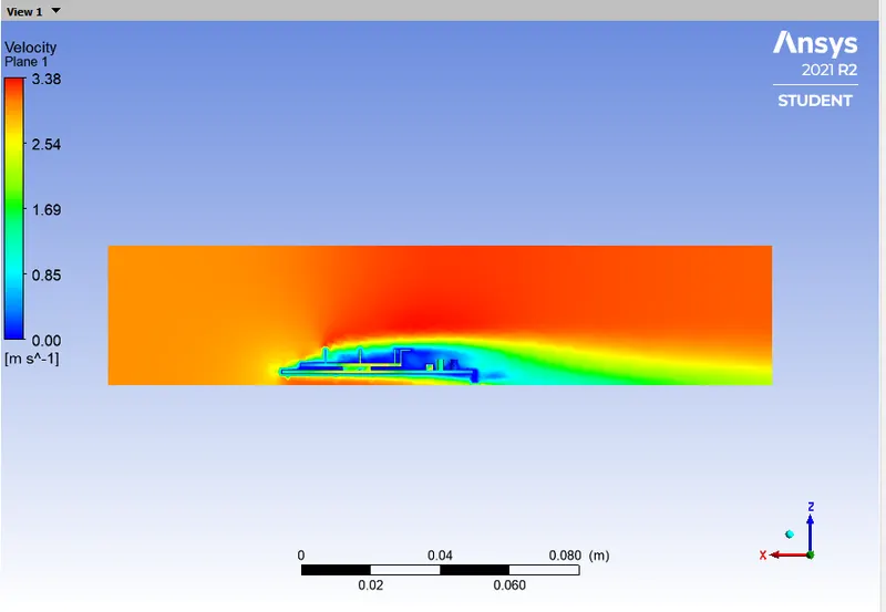
VELOCITY CONTOUR:

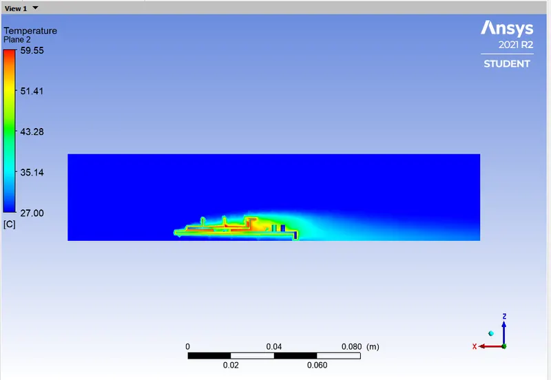
TEMPERATURE CONTOUR:

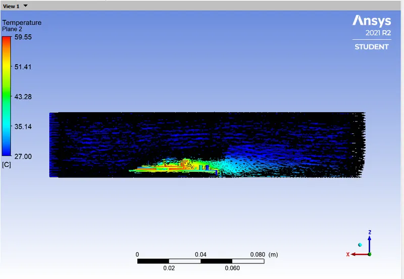
TEMPERATURE CONTOUR WITH VELOCITY VECTORS:

TEMPERATURE CONTOUR ON THE GRAPHICS CARD:

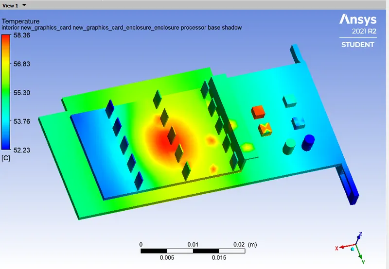
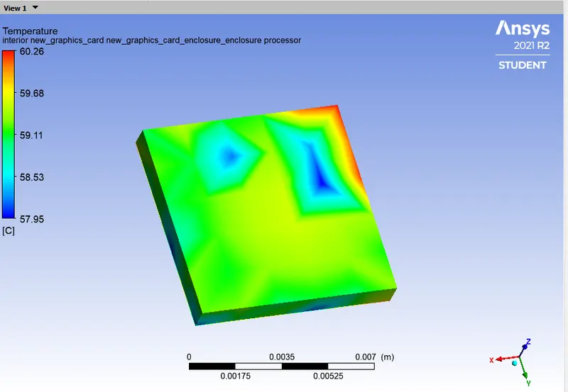
TEMPERATURE CONTOUR ON THE PROCESSOR:

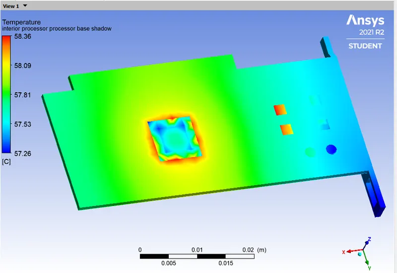
TEMPERATURE CONTOUR ON THE BASE:

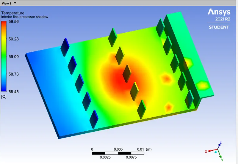
TEMPERATURE CONTOUR ON THE HEAT SINK:

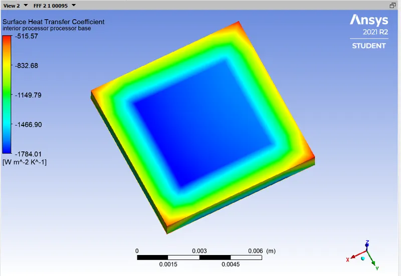
TEMPERATURE CONTOUR OF SURFACE HEAT TRANSFER COEFFICIENT OF THE PROCESSOR:

CASE - 4:

• Refined Mesh
• Mesh Element Size: 1.6 mm
• Total Elements: 499615
• Inlet Velocity: 5m/s

GEOMETRY:

• In Ansys Spaceclaim we need to enable the share in the topology box and perform the share operation from the workbench menu so that all the walls of the component share their common boundary and we will get a conformal mesh.

MESHING:

• As per trial error method we got the Mesh element size as 1.6mm as the best possible size as the total number of elements are 499615 which can be simulated without any problem.
• Here in meshing we need to properly name the components and faces as per required and check that after generation of mesh it generates conformal mesh.
• It's very important to have conformal mesh in this assignment so that the heat generated from the processor travels properly to the neighboring components so that the heat generated from it gets dissipated and we get the correct result from the simulation.

SETUP:

• In this assignment we are using the K-Omega SST turbulence model to run the simulation.
• We have to select proper material for different components of the graphics card.
• Processor: Titanium
• Base: Copper
• Heat Sink: Aluminum
• We have to define the heat generation source term for the processor that is 78125000 W/m^3.

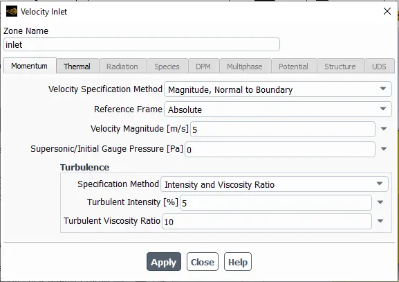
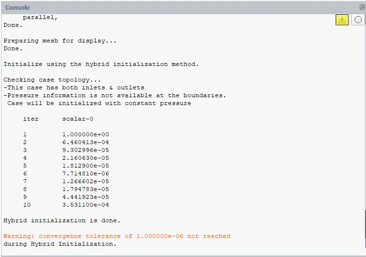
RESULTS:

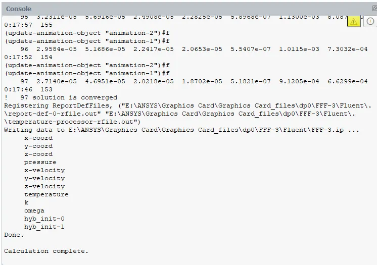
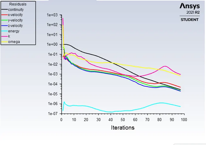
RESIDUALS:

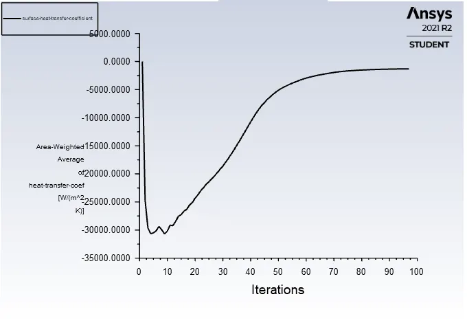
HEAT TRANSFER COEFFICIENT OF PROCESSOR:

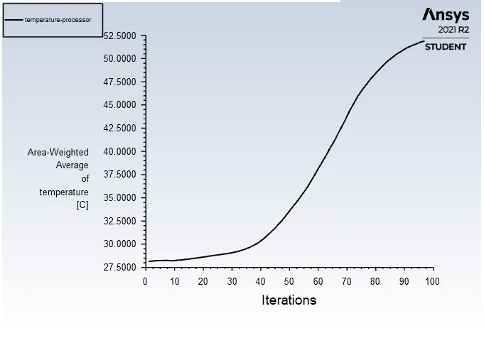
MAXIMUM TEMPERATURE OF PROCESSOR:

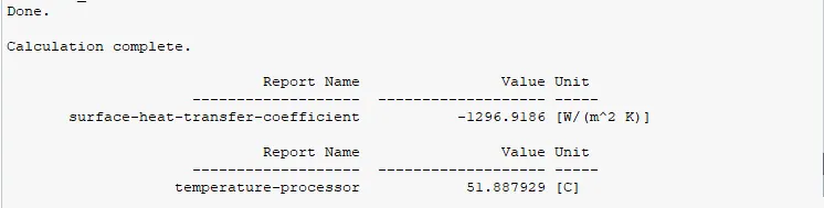
VALUES:

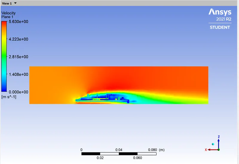
VELOCITY CONTOUR:

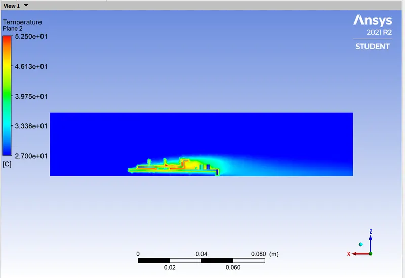
TEMPERATURE CONTOUR:

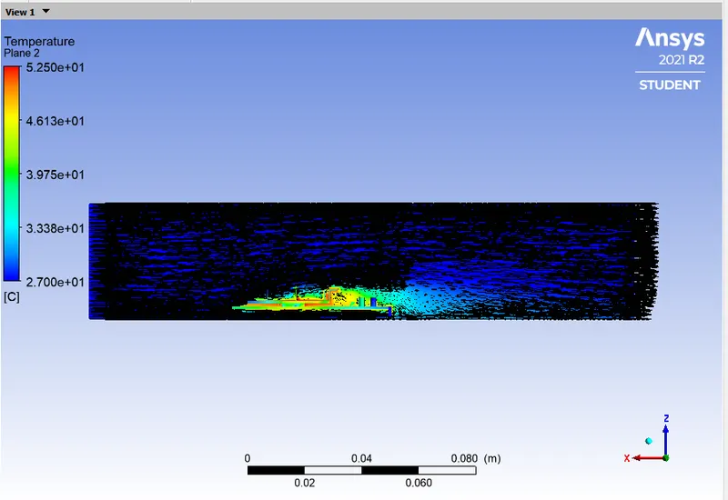
TEMPERATURE CONTOUR WITH VELOCITY VECTORS:

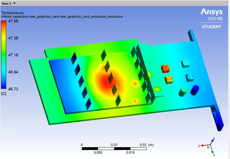
TEMPERATURE CONTOUR ON THE GRAPHICS CARD:

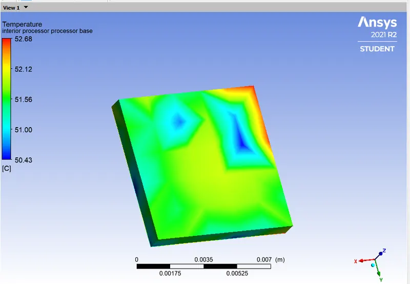
TEMPERATURE CONTOUR ON THE PROCESSOR:

TEMPERATURE CONTOUR ON THE BASE:

TEMPERATURE CONTOUR ON THE HEAT SINK:

TEMPERATURE CONTOUR OF SURFACE HEAT TRANSFER COEFFICIENT OF THE PROCESSOR:

TABULATION:

SL. NO	ELEMENT SIZE (mm)	TOTAL NUMBER OF ELEMENTS	VELOCITY (m/s)	HEAT TRANSFER COEFFICIENT OF PROCESSOR (W/m^2-K)	MAXIMUM TEMPERATURE OF PROCESSOR(C)
01.	10.289	83285	1	-485.27145	92.2783
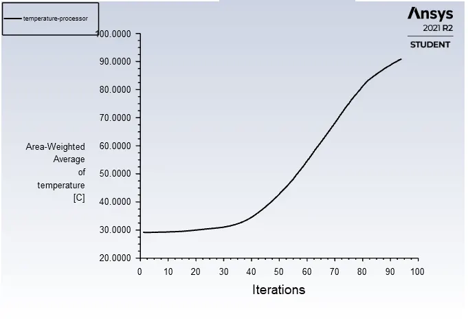
02.	1.6	499615	1	-496.59565	90.9196
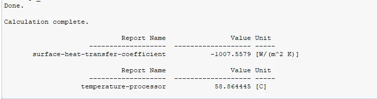
03.	1.6	499615	3	-1007.5579	58.8644
04.	1.6	499615	5	-1296.9186	51.8897

CONCLUSION:

• From the above assignment we learnt about the heat transfer in a Graphics Card.
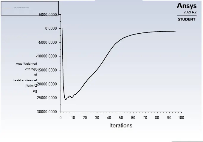
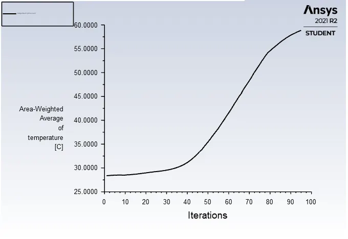
• We can observe that as the velocity of the inlet air increases the maximum temperature of the processor decreases and heat transfer coefficient of the processor increases. (Absolute value) (Negative sign depends upon dt).
• This happens because as the air velocity increases the Reynold's Number at that area increases which in turn increases the Nusselt Number, As the Nusselt Number increases the convective heat transfer coefficient increases.
• Also, as the inlet velocity of air increases the graphics card cools down faster this means that the heat transfer to the air is more. As it cools down faster so the maximum temperature drops down and as the heat transfer rate is faster to the surrounding so the heat transfer coefficient is more.
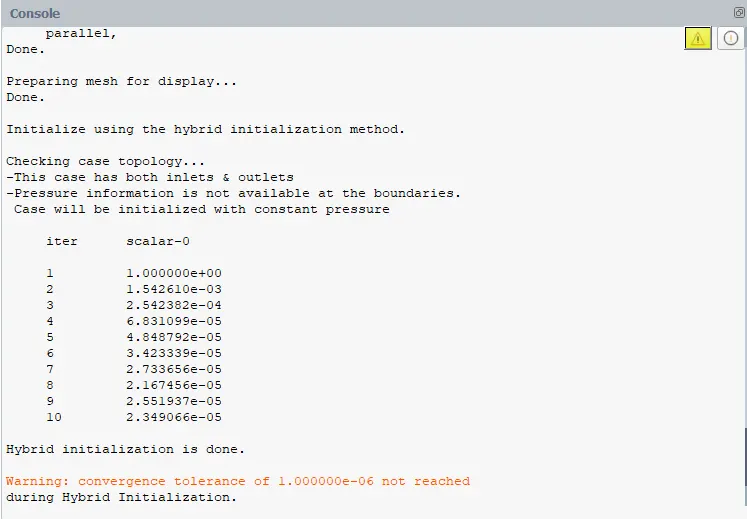
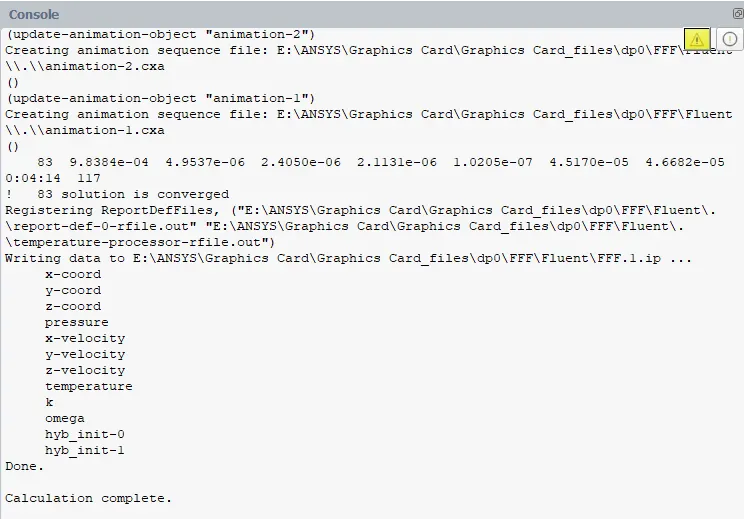
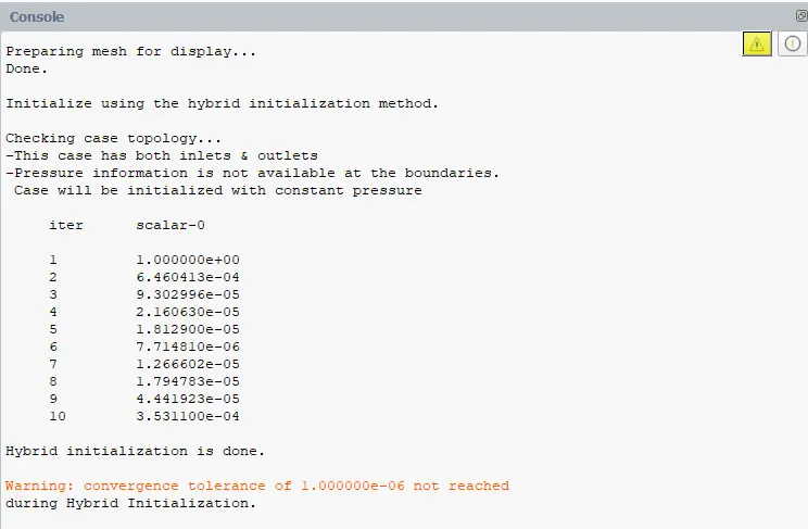
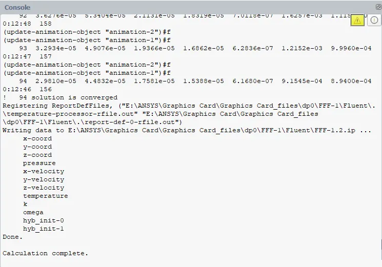
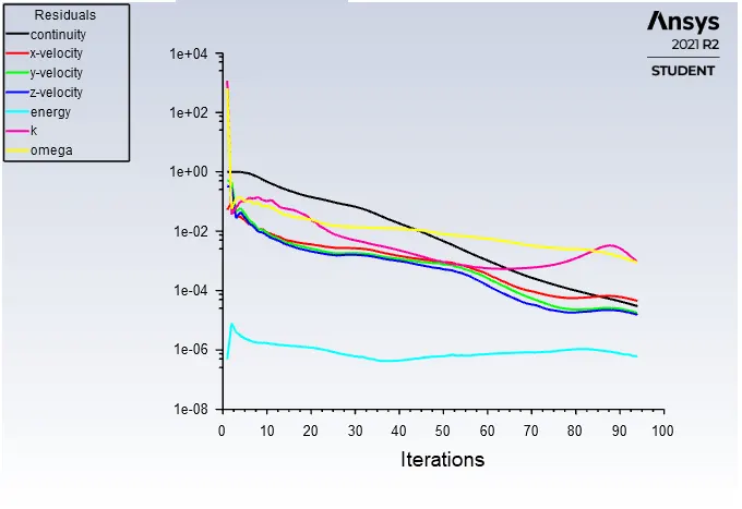
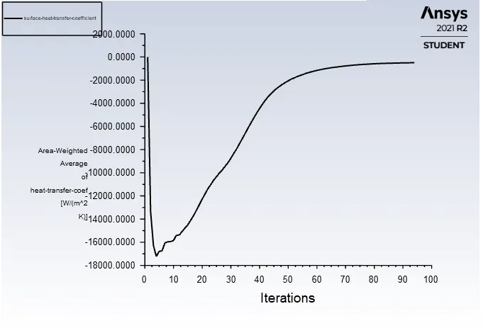
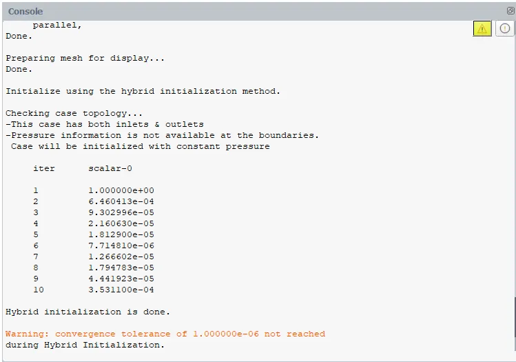
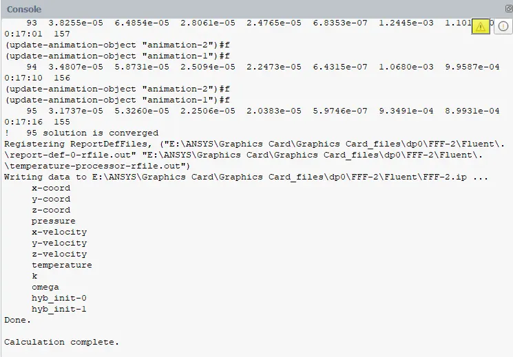
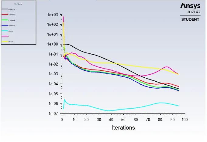
• From the above plots and the console images we can see that the solution has converged and also the heat transfer coefficient becomes constant. So, we can infer that the solution has converged.
• From the different temperature contours we can identify the hotspot zones of the graphics card.
• We can see that the temperature at the processor and the surrounding surfaces has the highest temperature.
• As our processor is the heat generating source and after that it conducts the heat generated to its nearby components, So the hotspot zones are all over nearby the processor only.
• The walls of the Graphics card base and the Heat Sink which share a common wall with the Processor has the highest temperature in that region and the temperature drops down as we go away from that region.