Final Project: Design of an Electric Vehicle

OBJECTIVE:

• To design an Electric Vehicle in Simulink which uses battery and a DC motor.
• To prepare a report about the model including the following:
  • System level configurations
  • Model parameters
  • Results
  • Conclusion

SOLUTION:

• An electric vehicle (EV) is a vehicle powered by an electric motor, instead of an internal combustion engine (ICE), and the motor is run using the power stored in the batteries. The batteries have to be charged frequently by plugging into any main (120 V or 240 V) supply. EV has a much longer history than most people realize. EVs were seen soon after Joseph Henry introduced the first DC-powered motor in 1830. The first known electric car was a small model built by Professor Stratingh in the Dutch town of Groningen in 1835. The first EV was built by in 1834 by Thomas Davenport in the U.S., followed by Moses Farmer, who built the first two-passenger EV in 1847. There were no rechargeable electric cells (batteries) at that time. An EV did not become a viable option until the Frenchmen Gaston Plante and Camille Faure respectively invented (1865) and improved (1881) the storage battery.
• EVs are known as zero emissions vehicles (ZEVs) and are much more environmentally friendly than gasoline- or LPG-powered vehicles. As EVs have fewer moving parts, maintenance is also minimal. With no engine there are no oil changes, tune-ups, or timing and there is no exhaust. EVs are also far more energy efficient than gasoline engines and they are very quiet in operation.

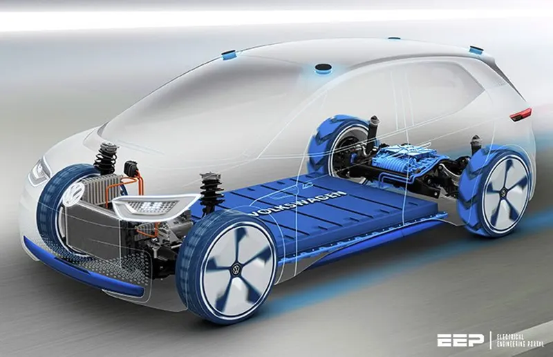
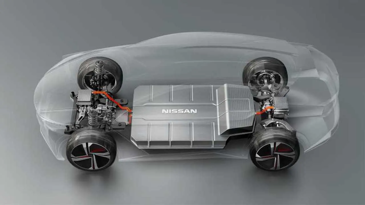
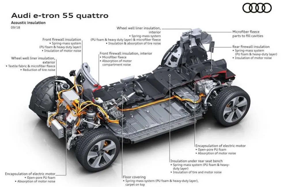
• EVs have been in continual use since the 1900s in various applications. Today these quiet vehicles with no tailpipe emissions are no longer limited to golf carts. New advances in battery technology, system integration, aerodynamics, and research and development by major vehicle manufacturers have led to the production of electric vehicles that will play a practical role on city streets. EVs don’t have ICEs in them. Instead, electrical energy is stored in a storage battery or ultracapacitor, converted from chemical energy in a fuel cell, or converted from mechanical energy in a flywheel. This electrical energy is used to power an electric motor, which then turns the wheels and provides propulsion. Since no fuel is burned in an EV, they don’t produce the pollution that ICE vehicles do. EVs are not new:
  The first automobiles to be built were all EVs, using energy stored in rudimentary lead acid batteries to drive DC electric motors. Only in the 1910s did gasoline-powered vehicles
  begin to make serious inroads in the automobile market.
• Unfortunately, EVs have a serious disadvantage that played a large role in the takeover by ICE vehicles: limited range. By limited range we mean that EVs could only travel on the order of 50 miles or so on a single charge, and that only under good conditions (lead-acid batteries lose energy capacity when they become cold, so in cold weather the range of a vehicle could be reduced by as much as 50% or even more). Also, recharging takes hours. ICE vehicles can go much farther on a tankful of gas and could be quickly refueled.
• Now, urban air quality issues, coupled with a rising awareness of the problems associated with the world’s (and particularly America’s) appetite for oil, have created interest in EVs. Power electronics have revolutionized motor drives, bringing within the realm of possibility electric drivetrains with extremely high performance, and the motors themselves have been improved, offering higher reliability and better performance with reduced cost. Unfortunately, the weak link in the chain remains — electrochemical batteries. There are some new battery chemistries floating around that offer good promise in terms of range, but none has the desired combination of three features: fast charging/discharging (high power density), large storage capacity (high energy density), and low cost. Traditional lead-acid batteries have been improved some over the years, but their energy and power densities remain disappointingly low, particularly when compared with gasoline.

MODELLING OF AN ELECTRIC VEHICLE IN SIMULINK:

VEHICLE BODY SUB-SYSTEM:

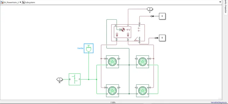
• In order to design an Electric Vehicle first we need to design the architecture of the vehicle.
• The architecture of the vehicle contains Tires, Vehicle Body, Simple Gear and an Inertia Shaft.
• Using the above blocks the architecture of the Vehicle body can be designed.
• First of all, all the tires are connected to the respective axle i.e. Front axle and Rear axle.
• Then all the Wheel hubs are connected to each other and then connected to the Hub port of the Vehicle body.
• The Normal forces on the wheel of the rear side is connected to the normal forces port of the rear wheels and the Normal forces on the wheel of the front side is connected to the normal forces port of the front side.
• A Simple gear block is then connected to the axle of the rear side wheels which makes the vehicle Rear Wheel drive.
• We can connect the gear box as per our requirement to make the vehicle Rear Wheel Drive, Front Wheel Drive or All Wheel Drive.
• The inertia shaft is then connected between the gear block and the rear wheel axle connection.
• As per our requirement we can provide the Inclination angle value, Wind speed value in the Vehicle body block and Slip value in the Tire block.
• The Input to the Gear block is the input port of the Sub-system and the Velocity port from the Vehicle body is the output of the Sub-system.

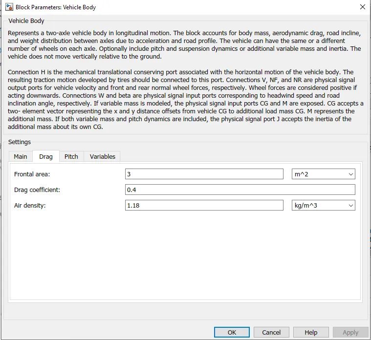
1. VEHICLE BODY BLOCK:

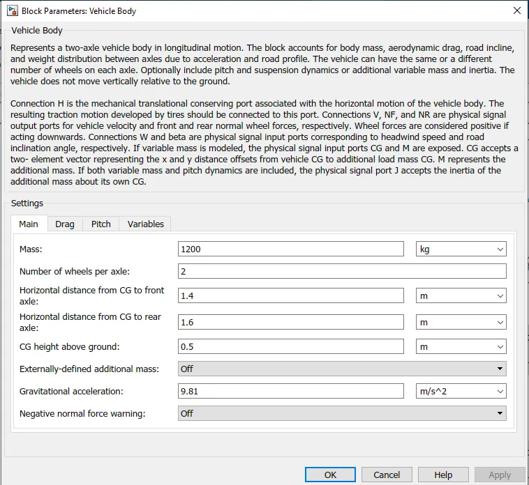
• Represents a two-axle vehicle body in longitudinal motion. The block accounts for body mass, aerodynamic drag, road incline, and weight distribution between axles due to acceleration and road profile. The vehicle can have the same or a different number of wheels on each axle. Optionally include pitch and suspension dynamics or additional variable mass and inertia. The vehicle does not move vertically relative to the ground.
• Connection H is the mechanical translational conserving port associated with the horizontal motion of the vehicle body. The resulting traction motion developed by tires should be connected to this port. Connections V, NF, and NR are physical signal output ports for vehicle velocity and front and rear normal wheel forces, respectively. Wheel forces are considered positive if acting downwards. Connections W and beta are physical signal input ports corresponding to headwind speed and road inclination angle, respectively. If variable mass is modeled, the physical signal input ports CG and M are exposed. CG accepts a two- element vector representing the x and y distance offsets from vehicle CG to additional load mass CG. M represents the additional mass. If both variable mass and pitch dynamics are included, the physical signal port J accepts the inertia of the additional mass about its own CG.

2. TIRES BLOCK:

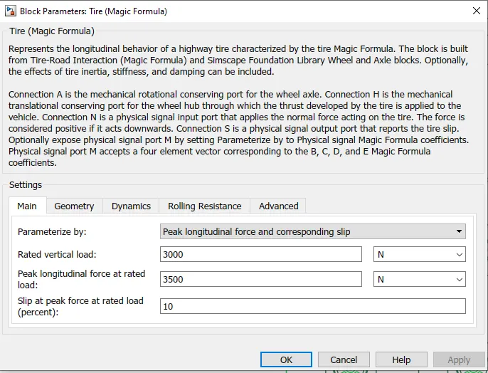
• Represents the longitudinal behavior of a highway tire characterized by the tire Magic Formula. The block is built from Tire-Road Interaction (Magic Formula) and Simscape Foundation Library Wheel and Axle blocks. Optionally, the effects of tire inertia, stiffness, and damping can be included.
• Connection A is the mechanical rotational conserving port for the wheel axle. Connection H is the mechanical translational conserving port for the wheel hub through which the thrust developed by the tire is applied to the vehicle. Connection N is a physical signal input port that applies the normal force acting on the tire. The force is considered positive if it acts downwards. Connection S is a physical signal output port that reports the tire slip. Optionally expose physical signal port M by setting Parameterize by to Physical signal Magic Formula coefficients. Physical signal port M accepts a four-element vector corresponding to the B, C, D, and E Magic Formula coefficients.

3. SIMPLE GEAR BLOCK:

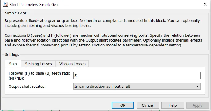
• Represents a fixed-ratio gear or gear box. No inertia or compliance is modeled in this block. You can optionally include gear meshing and viscous bearing losses.
• Connections B (base) and F (follower) are mechanical rotational conserving ports. Specify the relation between base and follower rotation directions with the Output shaft rotates parameter. Optionally include thermal effects and expose thermal conserving port H by setting Friction model to a temperature-dependent setting.

4. INERTIA BLOCK:

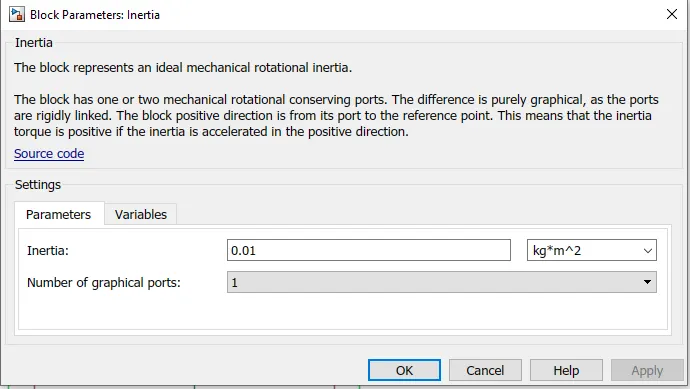
• The block represents an ideal mechanical rotational inertia.
• The block has one or two mechanical rotational conserving ports. The difference is purely graphical, as the ports are rigidly linked. The block positive direction is from its port to the reference point. This means that the inertia torque is positive if the inertia is accelerated in the positive direction.

MAIN SYSTEM:

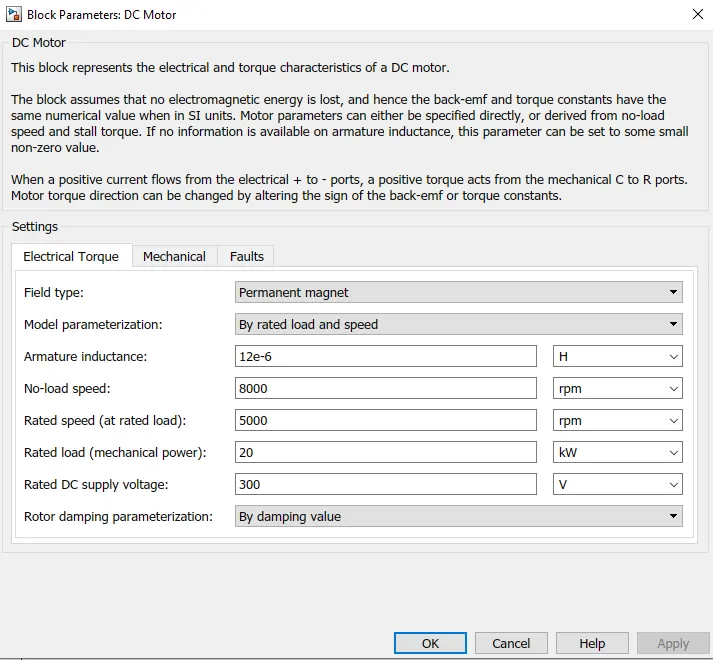
5. DC MOTOR BLOCK:

• A DC motor block is used to simulate the Electric Vehicle using different drive cycles.
• The R port of the DC Motor is connected to the Input of the Vehicle Sub-system and the C port of the DC Motor is connected to the Mechanical Rotational Reference

6. LONGITUDINAL DRIVER BLOCK:

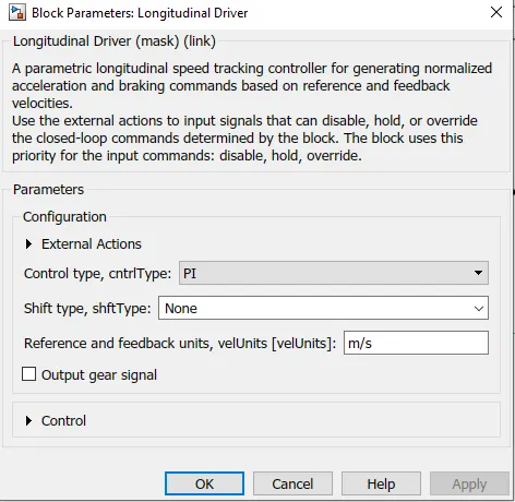
• A longitudinal driver block is used to generate acceleration and deceleration commands or signals based on the drive cycle input.
• A parametric longitudinal speed tracking controller for generating normalized acceleration and braking commands based on reference and feedback velocities.
• Use external actions to input signals that can disable, hold, or override the closed-loop commands determined by the block. The block uses this priority for the input commands: disable, hold, override.

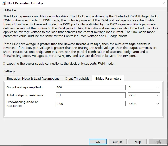
7. H-BRIDGE BLOCK:

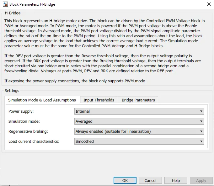
• This block represents an H-bridge motor drive. The block can be driven by the Controlled PWM Voltage block in PWM or Averaged mode. In PWM mode, the motor is powered if the PWM port voltage is above the Enable threshold voltage. In Averaged mode, the PWM port voltage divided by the PWM signal amplitude parameter defines the ratio of the on-time to the PWM period. Using this ratio and assumptions about the load, the block applies an average voltage to the load that achieves the correct average load current. The Simulation mode parameter value must be the same for the Controlled PWM Voltage and H-Bridge blocks.
• If the REV port voltage is greater than the Reverse threshold voltage, then the output voltage polarity is reversed. If the BRK port voltage is greater than the Braking threshold voltage, then the output terminals are short circuited via one bridge arm in series with the parallel combination of a second bridge arm and a freewheeling diode. Voltages at ports PWM, REV and BRK are defined relative to the REF port.
• If exposing the power supply connections, the block only supports PWM mode.

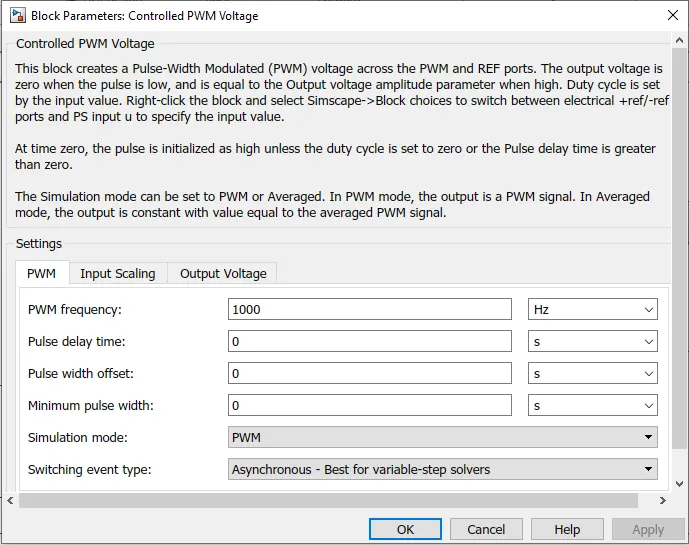
8. CONTROLLED PWM VOLTAGE BLOCK:

• This block creates a Pulse-Width Modulated (PWM) voltage across the PWM and REF ports. The output voltage is zero when the pulse is low, and is equal to the Output voltage amplitude parameter when high. Duty cycle is set by the input value. Right-click the block and select Simscape->Block choices to switch between electrical +ref/-ref ports and PS input u to specify the input value.
• At time zero, the pulse is initialized as high unless the duty cycle is set to zero or the Pulse delay time is greater than zero.
• The Simulation mode can be set to PWM or Averaged. In PWM mode, the output is a PWM signal. In Averaged mode, the output is constant with value equal to the averaged PWM signal.

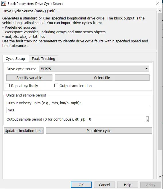
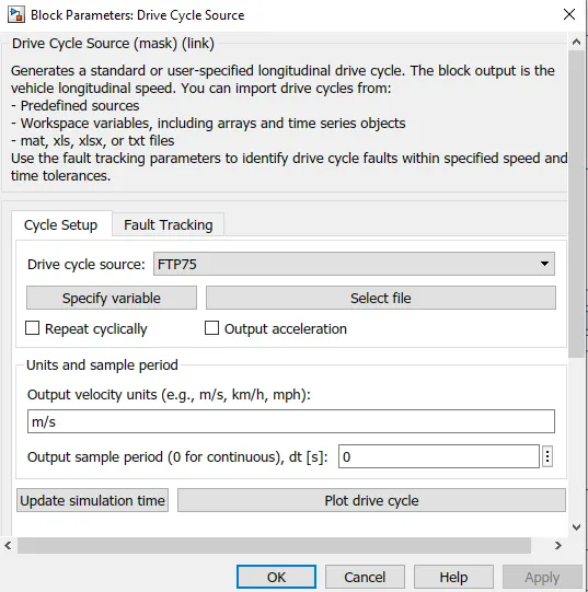
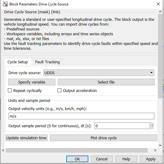
9. DRIVE CYCLE SOURCE BLOCK:

• Generates a standard or user-specified longitudinal drive cycle. The block output is the vehicle longitudinal speed. You can import drive cycles from:
  • Predefined sources
  • Workspace variables, including arrays and time series objects
  • mat, xls, xlsx, or txt files
• Use the fault tracking parameters to identify drive cycle faults within specified speed and time tolerances.

10. CONTROLLED VOLTAGE SOURCE:

• The block represents an ideal voltage source that is powerful enough to maintain the specified voltage at its output regardless of the current passing through it. The output voltage is V = Vs, where Vs is the numerical value presented at the physical signal port.

11. CURRENT SENSOR:

• The block represents an ideal current sensor, that is, a device that converts current measured in any electrical branch into a physical signal proportional to the current.
• Connections + and - are conserving electrical ports through which the sensor is inserted into the circuit. Connection I is a physical signal port that outputs current value.

12. CONTROLLED CURRENT SOURCE:

• The block represents an ideal current source that is powerful enough to maintain the specified current through it regardless of the voltage across it. The output current is I = Is, where Is is the numerical value presented at the physical signal port.

13. PS-SIMULINK CONVERTER BLOCK:

• Converts the input Physical Signal to a Simulink output signal.
• The unit expression in 'Output signal unit' parameter must match or be commensurate with the unit of the Physical Signal and determines the conversion from the Physical Signal to the Simulink output signal.
• 'Apply affine conversion' check box is only relevant for units with offset (such as temperature units).

14. SIMULINK-PS CONVERTER BLOCK:

• Converts the Simulink input signal to a Physical Signal.
• The unit expression in 'Input signal unit' parameter is associated with the Simulink input signal and determines the unit assigned to the Physical Signal.
• 'Apply affine conversion' check box is only relevant for units with offset (such as temperature units).
• If the selected solver requires input derivatives, you can either provide them explicitly through additional signal ports, or turn on input filtering to calculate time derivatives. The first-order filter provides one derivative, while the second-order filter provides the first and second derivatives. For piecewise-constant signals, you can also explicitly set the input derivatives to zero.

15. INTEGRATOR BLOCK:

• Continuous-time integration of the input signal.

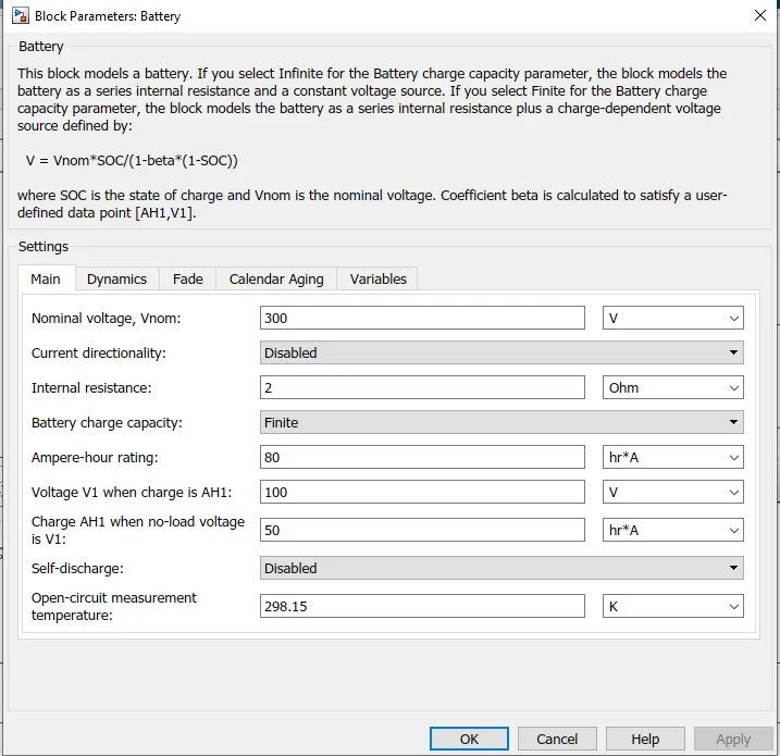
16. BATTERY:

• This block models a battery. If you select Infinite for the Battery charge capacity parameter, the block models the battery as a series internal resistance and a constant voltage source. If you select Finite for the Battery charge capacity parameter, the block models the battery as a series internal resistance plus a charge-dependent voltage source defined by:
• V = Vnom*SOC/(1-beta*(1-SOC))
• where SOC is the state of charge and Vnom is the nominal voltage. Coefficient beta is calculated to satisfy a user-defined data point [AH1,V1].

STATE OF CHARGE (SOC) ESTIMATION:

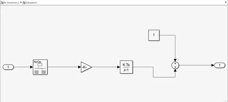
• To calculate the SOC output from the current sensor of the DC motor is taken as the Input.
• A Sub-system is created to estimate the state of charge of the Battery.
• Blocks used in the Sub-system to calculate the SOC is:
  • Rate Transition Block:
    • Handle data transfer between different rates and tasks.
    • The input from the current sensor is given to this block.
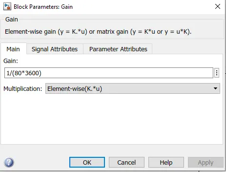
  • Gain Block:
    • Element-wise gain (y = K.*u) or matrix gain (y = K*u or y = u*K).
    • The formula used here is 1 / (80*3600).
    • Where 80 is the Ampere-Hour rating of the battery.
  • Discrete Time Integrator Block:
    • Discrete-time integration or accumulation of the input signal.
  • Constant Block:
    • Output is constantly specified by the 'Constant value' parameter. If 'Constant value' is a vector and 'Interpret vector parameters as 1-D' is on, treat the constant value as a 1-D array. Otherwise, output a matrix with the same dimensions as the constant value.
  • Adder Block:
    • Add or subtract inputs. Specify one of the following:
    • Character vector containing + or - for each input port, | for spacer between ports (e.g. ++|-|++)
    • Scalar, >= 1, specifies the number of input ports to be summed.
    • When there is only one input port, add or subtract elements over all dimensions or one specified dimension
• The output from the Adder block gives the State of Charge of the battery.

CONNECTIONS:

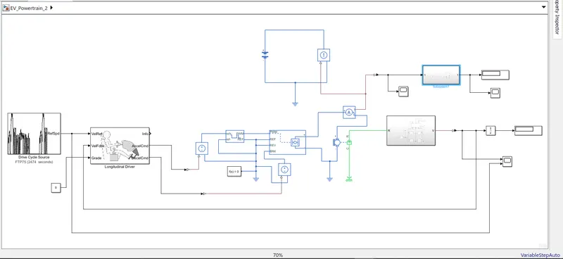
• The output from the Drive Cycle Source is connected to the Velocity Reference port of the Longitudinal Driver block.
• The output Velocity from the Vehicle body block or the Vehicle Sub-system is given as input to the Longitudinal driver block in the Velocity Feedback block using a PS-Simulink converter.
• The requirement of the velocity feedback is as per the velocity output from the vehicle and velocity requirement as per the drive cycle the Acceleration and Deceleration command will be given to the H-Bridge block.
• Then the acceleration command is fed to the Controlled PWM Voltage block using a controlled voltage source block by a Simulink-PS converter.
• Then the PWM signal from the controlled PWM voltage block is sent to the H-Bridge PWM port
• Then the deceleration command is fed to the H-Bridge block to the Brake port using a controlled voltage source block by a Simulink-PS converter.
• And all the other ports are connected as per the requirement and then connected to the Electrical reference that is ground.
• The Positive port of the H-Bridge is connected to the positive terminal of the DC motor through a Current sensor to measure the current in the DC motor.
• A Battery block is used to provide the necessary voltage and current to run the DC motor and is connected through a Controlled Current source.
• Both the Current sensor and the controlled Current Source are connected to supply the required current and voltage to the DC motor.
• Then one of the outputs of the Current sensor is provided as input to the SOC estimation Sub-system to calculate the State of Charge of the battery.
• As we know by integrating the velocity, we can calculate the actual distance travelled by the Vehicle.
• So a Integrator block is used to which the velocity output from the Vehicle body Sub-system is fed using a PS-Simulink converter and the actual travelled distance by the Electric Vehicle is calculated.
• Scopes and Display blocks are attached as per the requirement in order to vie the total distance covered by the Electric vehicle, The SOC of the Battery and the Current used by the DC Motor.

ELECTRIC VEHICLE MODELLING USING SIMULINK:

RESULTS:

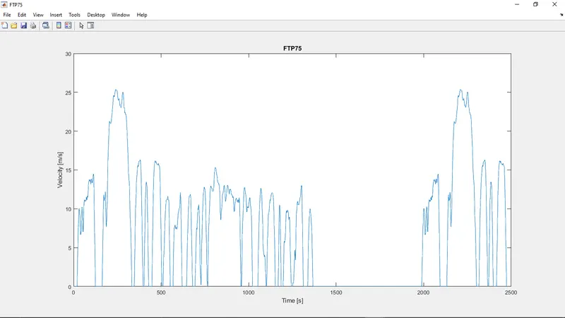
1. FTP-75:

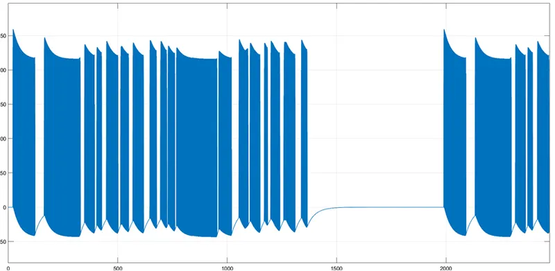
CURRENT SCOPE:

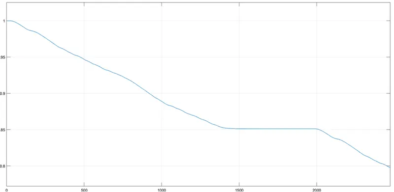
BATTERY SOC:

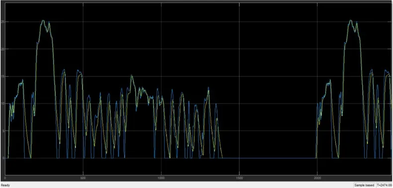
DISTANCE COVERED:

2. UDDS:

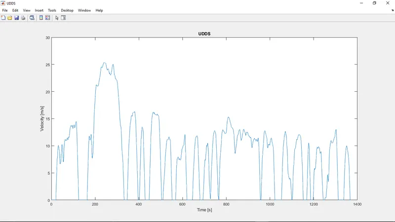
CURRENT SCOPE:

BATTERY SOC:

DISTANCE COVERED:

CONCLUSION:

• From the above assignment we learnt how to design an Electric Vehicle using Simulink.
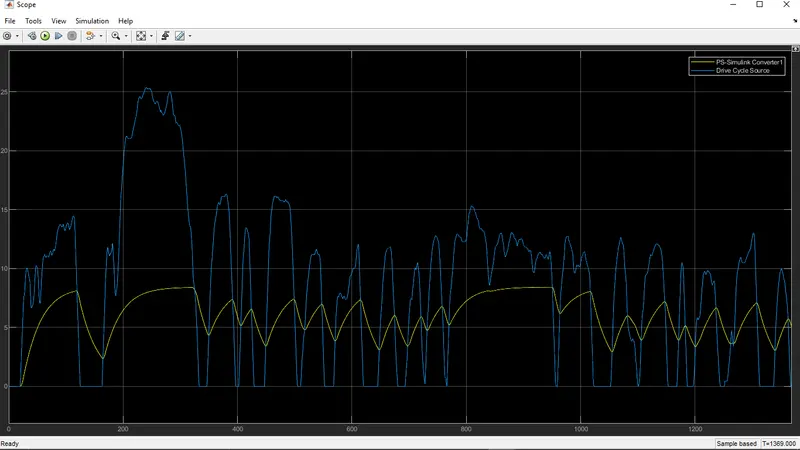
• We simulated our designed Electric Vehicle for drive cycle FTP-75 and UDDS and observed the results.
• From the distance scope we can observe that the Electric Vehicle powertrain followed the path of the Drive cycle we have used as the reference.
• We also observed the Current taken by the DC motor.
• We also observed the State of Charge of the battery at the end of the Drive Cycle.