Week 3.5 - Deriving 4th order approximation of a 2nd order derivative using Taylor Table method
The Analytical Function given in the question is : `exp(x)*cos(x)`
The Analytical derivative is: `-2*exp(x)*sin(x)`
CENTRAL DIFFERENCING:
For Fourth Order Approximation using Central Differencing method first we need to calculate the number of 'Nodes' to create the Numerical Boundary or Stencil.
According to the formula for Symmetrical or Central Differencing:
The order of accuracy P = Number of nodes in the stencil N - order of derivative Q + 1
Therefore, 4 = N - 2 + 1
N = 5
The number of nodes required for Central Differencing is 5.
So the formula to calculate the Fourth Order Approximation of a Second Order Derivative using Central Differencing is:
`a*f(x-2) + b*f(x-1) +c*f(x) + d*f(x+1) + e*f(x+2)`
To calculate 5 unknown variables 5 equations are required which we can form using Taylor Table
TAYLOR'S TABLE FOR CENTRAL DIFFERENCING:
f(x) dx*f'(x) dx^2*f''(x) dx^3*f'''(x) dx^4*f''''(x)
a(x-2) a -2a 4a/2 -8a/6 16a/24
b(x-1) b -b b/2 -b/6 b/24
c(x11) c 0 0 0 0
d(x+1) d d d/2 d/6 d/24
e(x+2) e 2e 4e/2 8e/6 16e/24
Forming the equations
a + b + c + d + e = 0 ----------------------------(1)
-2a - b + d + 2e = 0 ------------------------------(2)
4a + b + d + 4e = 2 ------------------------------(3)
-8a - b + d + 8e = 0 ------------------------------(4)
16a + b + d + 16e = 0 ----------------------------(5)
Writing the above equation in Matrix form:
A = `[[1,1,1,1,1],[-2 ,-1,0,1,2],[4 ,1 ,0 ,1 ,4],[-8,-1,0,1,8],[16,1,0,1,16]]`
X = `[[a],[b],[c],[d],[e]]`
B = `[[0],[0],[2],[0],[0]]`
As we know A*X = B
and X = inv(A)*B
Using Matrix Inversion we can easily calculate our unknown values
After Solving the above equation in Matlab we will get the values of our unknowns.
After that our equation becomes:
`(d^2f)/dx^2 = (a*f(x-2*dx) + b*f(x-1*dx) + c*f(x) + d*f(x+1*dx) + e*f(x+2*dx))/(dx^2))`
SKEWED DIFFERENCING:
For Fourth Order Approximation using Skewed RHS Differencing and Skewed LHS method first we need to calculate the number of 'Nodes' to create the Numerical Boundary or Stencil.
According to the formula for Symmetrical or Central Differencing:
The order of accuracy P = Number of nodes in the stencil N - order of derivative Q
Therefore, 4 = N - 2
N = 6
SKEWED RHS DIFFERENCING:
The number of nodes required for Central Differencing is 6.
So the formula to calculate the Fourth Order Approximation of a Second Order Derivative using Skewed RHS Differencing:
`a*f(x) + b*f(x+1) + c*f(x+2) + d*f(x+3) + e*f(x+4) + f*f(x+5)`
To calculate 6 unknown variables 6 equations are required which we can form using Taylor Table
TAYLOR'S TABLE FOR SKEWED RHS DIFFERENCING:
f(x) dx*f'(x) dx^2*f''(x) dx^3*f'''(x) dx^4*f''''(x) dx^5*f""'(x)
a(x) a 0 0 0 0 0
b(x+1) b b b/2 b/6 b/24 b/120
c(x+2) c 2c 4c/2 8c/6 16c/24 32c/120
d(x+3) d 3d 9d/2 27d/6 81 d/24 243d/120
e(x+4) e 4e 16e/2 64e/6 256e/24 1024e/120
f(x+5) f 5f 25f/2 125f/6 625f/24 3125f/120
From the above table we can get our 6 equations
a + b + c + d + e + f = 0 -------------------------(1)
b + 2c + 3d + 4e + 5f = 0 ------------------------(2)
b + 4c + 9d + 16e + 25f = 2 ---------------------(3)
b + 8c + 27d + 64e + 125f = 0 ------------------(4)
b + 16c + 81d + 256e + 625f = 0 ---------------(5)
b + 32c + 243d + 1024e + 3125f = 0 -----------(6)
Writing the above equation in Matrix form:
A =`[[1,1,1,1,1,1],[0,1,2,3,4,5],[0,1,4,9,16,25],[0,1,8,27,64,125],[0,1,16,81,256,625],[0,1,32,243,1024,3125]]`
X = `[[a],[b],[c],[d],[e],[f]]`
B = `[[0],[0],[2],[0],[0],[0]]`
As we know A*X = B
and X = inv(A)*B
Using Matrix Inversion we can easily calculate our unknown values
After Solving the above equation in Matlab we will get the values of our unknowns.
After that our equation becomes:
`(d^2f)/dx^2 = (a*f(x) + b*f(x+1*dx) + c*f(x+2*dx) + d*f(x+3*dx) + e*f(x+4*dx) + f*f(x+5*dx))/(dx^2)`
SKEWED LHS DIFFERENCING:
The formula to calculate the Fourth Order Approximation of a Second Order Derivative using Skewed LHS Differencing:
`a*f(x) + b*f(x-1) + c*f(x-2) + d*f(x-3) + e*f(x-4) + f*f(x-5)`
To calculate 6 unknown variables 6 equations are required which we can form using Taylor Table
TAYLOR'S TABLE FOR SKEWED RHS DIFFERENCING:
f(x) dx*f'(x) dx^2*f''(x) dx^3*f'''(x) dx^4*f''''(x) dx^5*f""'(x)
a(x) a 0 0 0 0 0
b(x-1) b -b b/2 -b/6 b/24 -b/120
c(x-2) c -2c 4c/2 -8c/6 16c/24 -32c/120
d(x-3) d -3d 9d/2 -27d/6 81 d/24 -243d/120
e(x-4) e -4e 16e/2 -64e/6 256e/24 -1024e/120
f(x-5) f -5f 25f/2 -125f/6 625f/24 -3125f/120
From the above table we can get our 6 equations
a + b + c + d + e + f = 0 -------------------------(1)
b + 2c + 3d + 4e + 5f = 0 ------------------------(2)
b + 4c + 9d + 16e + 25f = 2 ---------------------(3)
b + 8c + 27d + 64e + 125f = 0 ------------------(4)
b + 16c + 81d + 256e + 625f = 0 ---------------(5)
b + 32c + 243d + 1024e + 3125f = 0 -----------(6)
Writing the above equation in Matrix form:
A =`[[1,1,1,1,1,1],[0,1,2,3,4,5],[0,1,4,9,16,25],[0,1,8,27,64,125],[0,1,16,81,256,625],[0,1,32,243,1024,3125]]`
X = `[[a],[b],[c],[d],[e],[f]]`
B = `[[0],[0],[2],[0],[0],[0]]`
As we know A*X = B
and X = inv(A)*B
Using Matrix Inversion we can easily calculate our unknown values
After Solving the above equation in Matlab we will get the values of our unknowns.
After that our equation becomes:
`(d^2f)/dx^2 = (a*f(x) + b*f(x-1*dx) + c*f(x-2*dx) + d*f(x-3*dx) + e*f(x-4*dx) + f*f(x-5*dx))/(dx^2)`
SOLVING THE ABOVE USING MATLAB
1.FUNCTION TO EVALUATE CENTRAL DIFFERENCING:
function out_1 = fourth_order_approximation_central(x,dx)

Analytical_Second_Order_Derivative =  -2*exp(x)*sin(x);

A(1,:) = [1 1 1 1 1];
A(2,:) = [-2 -1 0 1 2];
A(3,:) = [4 1 0 1 4];
A(4,:) = [-8 -1 0 1 8];
A(5,:) = [16 1 0 1 16];

B = [0 0 2 0 0]';

X = inv(A)*B;

% Fourth Order Approximation using Central Differencing

fourth_order_approximation_1 = (X(1,1)*exp(x-2*dx)*cos(x-2*dx) + X(2,1)*exp(x-1*dx)*cos(x-1*dx) + X(3,1)*exp(x)*cos(x) + X(4,1)*exp(x+1*dx)*cos(x+1*dx) + X(5,1)*exp(x+2*dx)*cos(x+2*dx))/(dx)^2;

out_1 = abs(fourth_order_approximation_1 - Analytical_Second_Order_Derivative);

end
2.FUNCTION TO EVALUATE SKEWED RHS DIFFERENCING:
function out_2 = fourth_order_approximation_skewed_rhs(x,dx)

Analytical_Second_Order_Derivative =  -2*exp(x)*sin(x);

C(1,:) = [1 1 1 1 1 1];
C(2,:) = [0 1 2 3 4 5];
C(3,:) = [0 1 4 9 16 25];
C(4,:) = [0 1 8 27 64 125];
C(5,:) = [0 1 16 81 256 625];
C(6,:) = [0 1 32 243 1024 3125];

D = [0 0 2 0 0 0]';

Y = inv(C)*D;

% Fourth Order Approximation using Skewed RHS Differencing

fourth_order_approximation_2 = (Y(1,1)*exp(x)*cos(x) + Y(2,1)*exp(x+1*dx)*cos(x+1*dx) + Y(3,1)*exp(x+2*dx)*cos(x+2*dx) + Y(4,1)*exp(x+3*dx)*cos(x+3*dx) + Y(5,1)*exp(x+4*dx)*cos(x+4*dx) + Y(6,1)*exp(x+5*dx)*cos(x+5*dx))/(dx)^2;

out_2 = abs(fourth_order_approximation_2 - Analytical_Second_Order_Derivative);

end
3. FUNCTION TO EVALUATE SKEWED LHS DIFFERENCING:
function out_3 = fourth_order_approximation_skewed_lhs(x,dx)

Analytical_Second_Order_Derivative =  -2*exp(x)*sin(x);

C(1,:) = [1 1 1 1 1 1];
C(2,:) = [0 1 2 3 4 5];
C(3,:) = [0 1 4 9 16 25];
C(4,:) = [0 1 8 27 64 125];
C(5,:) = [0 1 16 81 256 625];
C(6,:) = [0 1 32 243 1024 3125];

D = [0 0 2 0 0 0]';

Y = inv(C)*D;

% Fourth Order Approximation using Skewed LHS Differencing

fourth_order_approximation_3 = (Y(1,1)*exp(x)*cos(x) + Y(2,1)*exp(x-1*dx)*cos(x-1*dx) + Y(3,1)*exp(x-2*dx)*cos(x-2*dx) + Y(4,1)*exp(x-3*dx)*cos(x-3*dx) + Y(5,1)*exp(x-4*dx)*cos(x-4*dx) + Y(6,1)*exp(x-5*dx)*cos(x-5*dx))/(dx)^2;

out_3 = abs(fourth_order_approximation_3 - Analytical_Second_Order_Derivative);

end
MAIN PROGRAM TO EVALUATE THE ABOVE QUESTION:
% Numerical Discretization
close all
clear all
clc

% Analytical Derivative
% Analytical Function = exp(x)*cos(x)

x = pi/4;
dx = linspace(pi/4,pi/40,40);

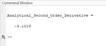
Analytical_Second_Order_Derivative =  -2*exp(x)*sin(x)

% Numerical Derivative
% Fourth Order Approximation of Second order Derivative


n_x = length(dx);

for i=1:n_x

    error_1(i) = fourth_order_approximation_central(x,dx(i));

    error_2(i) = fourth_order_approximation_skewed_rhs(x,dx(i));

    error_3(i) = fourth_order_approximation_skewed_lhs(x,dx(i));

end

figure(1)

plot(dx,error_1,'r')
hold on
plot(dx,error_2,'b')
hold on
plot(dx,error_3,'g')
xlabel('dx')
ylabel('Error')
legend('Central Differencing','Skewed RHS Differencing','Skewed LHS Differencin')

figure(2)
loglog(dx,error_1,'r')
hold on
loglog(dx,error_2,'b')
hold on
loglog(dx,error_3,'g')
xlabel('dx')
ylabel('Error')
legend('Central Differencing','Skewed RHS Differencing','Skewed LHS Differencin')
First we have defined 3 functions to calculate the fourth order approximation by central differencing, skewed rhs differencing, skewed lhs differencing.
Inside each function we have called the value of x and dx.
Then we have defined the Analytical Derivative of the above question.
After that to solve the Taylor's series table we have used Matrix Inversion method. So we have given the input of all coefficients in matrix format and then calculated the value of unknowns using Matrix Inversion Method.
After calculating the unknowns we have directly used matrix indices to calculate the respective approximations according to its formulae.
After that error is calculated with respect to the Analytical Derivative.
In the main function first we have defined the values of x and dx that will be used by each function.
Then we have defined the Analytical Derivative to display as the output.
Then we have calculated the total length of dx that is to be used by the for loop.
To calculate for different values of dx we need to write an 'For loop' so that for each value of dx the command will iterate and calculate the errors.
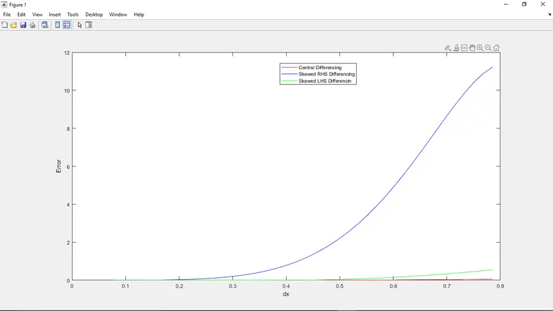
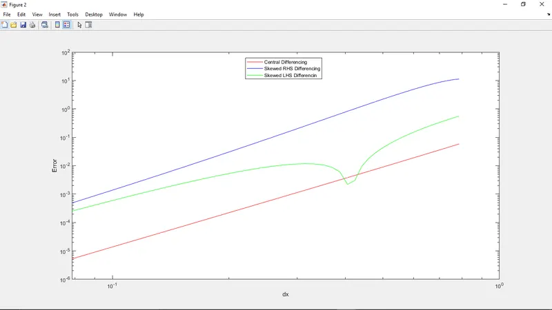
Then we have plotted 2 different types of graphs in order to study the trend of different type of differencing method to calculate Fourth order approximation of Second order derivative.
OUTPUT/GRAPHS:
CONCLUSION:
1. From the above graphs we can conclude that the Central Differencing method has the least errors as it uses points from both sides while in RHS or LHS differencing method it uses points from one side only.
The Skewed differencing method is useful
1.where points are given at only one side. As Central Differencing method uses points from both sides it cannot evaluate if points are given at one side only, there Skewed Differencing method will be very useful.
2. At boundary conditions Central Differencing cannot be used as it will have points on only side whereas Skewed Difference method can easily evaluate it by taking the points of single side only.
These are the cases where a Skewed Differencing method can really be useful.