Week 5.1 - Mid term project - Solving the steady and unsteady 2D heat conduction problem
1. STEADY STATE ANALYSIS:
The Steady State 2-Dimensional Heat Conduction Equation is:
`(partial^2T)/(partialx^2) + (partial^2T)/(partialy^2) = 0`
This equation can be further simplified by applying central diffrencing to both the Spatial Terms as:
`(T_R - 2*T_P + T_L)/(dx^2) + (T_B - 2*T_P + T_B)/(dy^2) = 0`
`T_p =1/ 2*((dx^2*dy^2)/(dx^2 + dy^2))*((T_L+T_R)/dx^2 + (T_B+T_T)/dy^2)`
So 'k' can be written as
`k = 2*((dx^2 + dy^2)/(dx^2*dy^2))`
`T_L =` Point to the left hand side of the present node = T(i-1,j)
`T_R =` Point to the right hand side of the present node = T(i+1,j)
`T_B =` Point to the bottom side of the present node = T(i,j-1)
`T_T =` Point to the top side of the present node = T(i,j+1)
`T_P =` Point at the present node = T(i,j)
The above equation can be solved by different splitting Iterative Methods:
1. JACOBI METHOD
2.GAUSS SIEDEL METHOD
3.SUCCESSIVE OVER RELAXATION METHOD
MATLAB PROGRAM TO EVALUATE ALL THE THREE METHODS:
% Steady State Analysis for 2D Heat Conduction

% Jacobi Method

clear all
close all
clc

% Domain Length
L_x = 1;
L_y = L_x;

% Number of Nodes
nx = 10;
ny = nx;

x = linspace(0,1,nx);
y = linspace(0,1,ny);

dx = L_x/(nx-1);
%dx_1 = x(2)-x(1);

dy = L_y/(ny-1);
%dy_1 = y(2)-y(1);

T = 300*ones(nx,ny);

% Boundary Conditions
T(1,:) = 600;
T(:,1) = 400;
T(:,end) = 800;
T(end,:) = 900;

% Corner Conditions
T(1,1) = 500;
T(1,end) = 700;
T(end,1) = 650;
T(end,end) = 850;

Told = T;
T_initial = T;

error = 10e10;

tol = 1e-4;

prompt = ('Enter the Solver Required ')
iterative_solver = input(prompt);

% Jacobi Solver

if iterative_solver==1
    j_iter = 1;
    tic
    while(error>tol)

        for i=2:nx-1
            for j=2:ny-1

                k = 2*((dx^2 + dy^2)/(dx^2*dy^2));
                term_1 = (Told(i-1,j) + Told(i+1,j))/(dx^2);
                term_2 = (Told(i,j-1) + Told(i,j+1))/(dy^2);
                T(i,j) = (term_1 + term_2)/k;

%                 T(i,j) = ((Told(i-1,j) + Told(i+1,j))/(dx^2) + (Told(i,j-1) + Told(i,j+1))/(dy^2))/k;

            end
        end

        error = max(max(abs(Told-T)));
        Told = T;
        j_iter = j_iter + 1;

        time_1 = toc;
    end

    figure(1)

    contourf(x,y,T,'ShowText','on')
    c = colorbar;
    c.Label.String = 'Temperature (K)'
    set(gca,'YDIR','reverse')
    colormap(jet)
    title_text=sprintf('Iteration Number = %d',j_iter);
    xlabel('X axis')
    ylabel('Y axis')
     s_t = sprintf('Simulation Time = %d secs',time_1);
    title(title_text,s_t)
end


% Gauss Siedel Method

% Gauss Siedel Solver

if iterative_solver==2
    gs_iter = 1;
    tic
    while(error>tol)

        for j=2:ny-1
            for i=2:nx-1

                k = 2*((dx^2 + dy^2)/(dx^2*dy^2));
                term_1 = (T(i-1,j) + T(i+1,j))/(dx^2);
                term_2 = (T(i,j-1) + T(i,j+1))/(dy^2);
                T(i,j) = (term_1 + term_2)/k;

%                 T(i,j) = ((T(i-1,j) + T(i+1,j))/(dx^2) + (T(i,j-1) + T(i,j+1))/(dy^2))/k;

            end
        end

        error = max(max(abs(Told-T)));
        Told = T;
        gs_iter = gs_iter + 1;

        time_2 = toc;
    end

    figure(2)

    contourf(x,y,T,'ShowText','on')
    c = colorbar;
    c.Label.String = 'Temperature (K)'
    set(gca,'YDIR','reverse')
    colormap(jet)
    title_text=sprintf('Iteration Number = %d',gs_iter);
    xlabel('X axis')
    ylabel('Y axis')
    s_t = sprintf('Simulation Time = %d secs',time_2);
    title(title_text,s_t)
end


% SOR Method

% SOR Solver
omega = 1.2;

if iterative_solver==3
    sor_iter = 1;
    tic
    while(error>tol)

        for j=2:ny-1
            for i=2:nx-1

                k = 2*((dx^2 + dy^2)/(dx^2*dy^2));
                term_1 = (T(i-1,j) + T(i+1,j))/(dx^2);
                term_2 = (T(i,j-1) + T(i,j+1))/(dy^2);
                T(i,j) = (1-omega)*Told(i,j) + omega*((term_1 + term_2)/k);

%                 T(i,j) = ((T(i-1,j) + T(i+1,j))/(dx^2) + (T(i,j-1) + T(i,j+1))/(dy^2))/k;

            end
        end

        error = max(max(abs(Told-T)));
        Told = T;
        sor_iter = sor_iter + 1;

        time_3 = toc;
    end

    figure(3)

    contourf(x,y,T,'ShowText','on')
    c = colorbar;
    c.Label.String = 'Temperature (K)'
    set(gca,'YDIR','reverse')
    colormap(jet)
    title_text=sprintf('Iteration Number = %d',sor_iter);
    xlabel('X axis')
    ylabel('Y axis')
    s_t = sprintf('Simulation Time = %d secs',time_3);
    title(title_text,s_t)

end
First we have defined all our variables and constants that are required to solve this problem.
As the above equation contains space values in both x and y direction so we need to define the values both in x and y direction.
First we have specified Domain Length, No of nodes and using the above length and grids we have ceated a matrix of some grid space.
After that we have calculate our grid spacing both in x and y directions.
Then we have formed our Temperature matrix using the given conditions of Top, Bottom, Left and Right sides, and we have calculated the corner values of the matrix by taking the average of the nearest values.
We have made the copies of Temperature matrix which will be used later on.
Then we have defined our values for error and tolerance so as to compare between them so that our loops will run untill the desired tolerance value is achieved.
After that we have used a prompt command that will take input from the user in-order to ask for which solver to run and as per the user it will show the plots.
i.e. 1- Jacobi Method
2- Gauss Siedel Method
3- SOR Method
1.JACOBI METHOD
In Jacobi method we have written a if statement that will be used to decide which method to follow according to the user input and then we have included a variable to count the total number of iterations.
Then we have written our Convergence Loop using While command which will run untill the comparision is made false.
After that we have written our formula to calculate the value of T by using the old values of T by using 2 for loops to represent both x and y direction.
After ending the for loop we have calculated the value of error which will be read by the while command to iterate the next loop, and we have updated the old value of T with the new value that we achieved.
After the solution gets stable we have plotted our graph showing the trend and total number of iterations taken to give the stable solution.
2.GAUSS SIEDEL METHOD
All the process followed in jacobi method are the exact same the only difference is that instead of using the old values of T we will be using the updated values of T.
All the rest Procedure are same.
3.SOR METHOD
In this method we have to introduce a new variable called omega because this method helps us to achieve the steady state at a faster rate. It acts like a catalyst to solve the equation.
FORMULA for SOR Method:
T(i,j) = (1 - omega)*Told(i,j) + omega*(T(Gauss Siedel Method) / T(Jacobi Method))
Here the Value of omega should be 1.1 or 1.2
PLOTS:
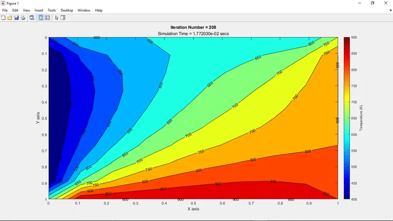
1. JACOBI METHOD
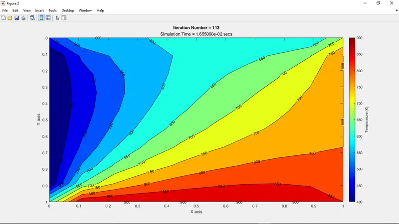
2. GAUSS SIEDEL METHOD:
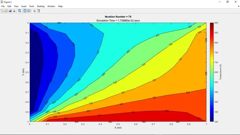
3. SOR METHOD
CONCLUSION;
From the above contour plots we can conclude that all the three methods have achieved the steady state but Jacobi Method has taken more number of Iterations than Gauss Siedel Method and SOR Method and Gauss Siedel Method has taken more number of Iterations than SOR method.
Number of Iterations= Jacobi(208) > Gauss Siedel(112) > SOR(76)
TRANSIENT STATE ANALYSIS OF 2D HEAT CONDUCTION EQUATION
The Transient State 2-Dimensional Heat Conduction Equation is:
`(partialT)/(partialt) + alpha*((partial^2T)/(partialx^2) + (partial^2T)/(partialy^2)) = 0`
This equation can be solved by both Implicit and Explicit scheme.
In Explicit Method we find the value of Temperature at (n+1) node by considering the values of temperature at the nodes that are already known i.e at T(n)
Whereas in Implicit Method we find the value of Temperature at (n+1) node by considering the values of temperature at the same (n+1) node.
Formula to calculate by Explicit Scheme:
Applying Forward Differencing to the Time Derivative terms and Central Differencing to the Spatial Terms
`(T_P^(n+1) - T_P^n)/dt = alpha*((T_R - 2*T_P + T_L)/dx^2+((T_T - 2*T_P + T_B)/(dy^2))^n`
`T_P^(n+1) =T_P^n+ dt*alpha*((T_R - 2*T_P + T_L)/dx^2+((T_T - 2*T_P + T_B)/(dy^2))^n`
`T_P^(n+1) =T_P^n+ k1*(T_R - 2*T_P + T_L)+k2*(T_T - 2*T_P + T_B)`
Where
`k1 = alpha*(dt/dx^2)`
`k2 = alpha*(dt/dy^2)`
Here k1 and k2 are the CFL numbers and also
The total value of CFL number must be less than equal to 0.5
i.e `CFL_T <= 0.5`
i.e `CFL_x + CFL_y <= 0.5`
We are calculating the value of T at (n+1) time node by using the values of T at 'n' node.
So here we have 1 unknown value and rest are known values, So for this scheme we can directly calculate using the above formula without doing iterative methods.
MATLAB PROGRAM TO EVALUATE THE ABOVE :
% Transient State Analysis for 2D Heat Conduction

% Explicit Method

clear all
close all
clc

% Domain Length
L_x = 1;
L_y = L_x;

% Number of Nodes
nx = 10;
ny = nx;

x = linspace(0,1,nx);
y = linspace(0,1,ny);

dx = L_x/(nx-1);
%dx_1 = x(2)-x(1);

dy = L_y/(ny-1);
%dy_1 = y(2)-y(1);

T = 300*ones(nx,ny);

% Boundary Conditions
T(1,:) = 600;
T(:,1) = 400;
T(:,end) = 800;
T(end,:) = 900;

% Corner Conditions
T(1,1) = 500;
T(1,end) = 700;
T(end,1) = 650;
T(end,end) = 850;

Told = T;
T_initial = T;

error = 10e10;

tol = 1e-4;

dt = 0.0001;

alpha = 1.4;

k1 = alpha*(dt/dx^2);
k2 = alpha*(dt/dy^2);

iter = 1;

% Time Loop
for t=1:1500

    tic
    % Space Loop

    for i=2:nx-1
        for j=2:ny-1

            term_1 = (Told(i-1,j) - 2*Told(i,j) + Told(i+1,j));
            term_2 = (Told(i,j-1) - 2*Told(i,j) + Told(i,j+1));
            T(i,j) = Told(i,j) + k1*term_1 + k2*term_2;

        end
    end

    Told = T;
    iter = iter+1;
    time_1 = toc;


end

        figure(1)

    contourf(x,y,T,'ShowText','on')
    c = colorbar;
    c.Label.String = 'Temperature (K)'
    set(gca,'YDIR','reverse')
    colormap(jet)
    title_text=sprintf('Iteration Number = %d',iter);
    xlabel('X axis')
    ylabel('Y axis')
     s_t = sprintf('Simulation Time = %d secs',time_1);
    title(title_text,s_t)
Procedure is same as the above methods the only change is as there is Time derivative so we need to calculate the Values of temperature for different Time Intervals.
So there will be a Time loop before the for loops and as we are not doing the Iterative methods so there will not be any Convergence loop i.e while loop.
We have to define the values of k1 and k2 and we should update the values of Told outside the for loops but inside the Time loop so that to calculate for different spacial nodes it will take the updated values of Temperature(T).
We must define the value of 'alpha' as 1.4 or 1.5. and also while defining dt and dx we must keep in mind that we must define such values so that 'k1+k2' must be less than or equal to 0.5.
After that we plot the contour graph to see the trend of the solution or stability of the solution.
PLOT:
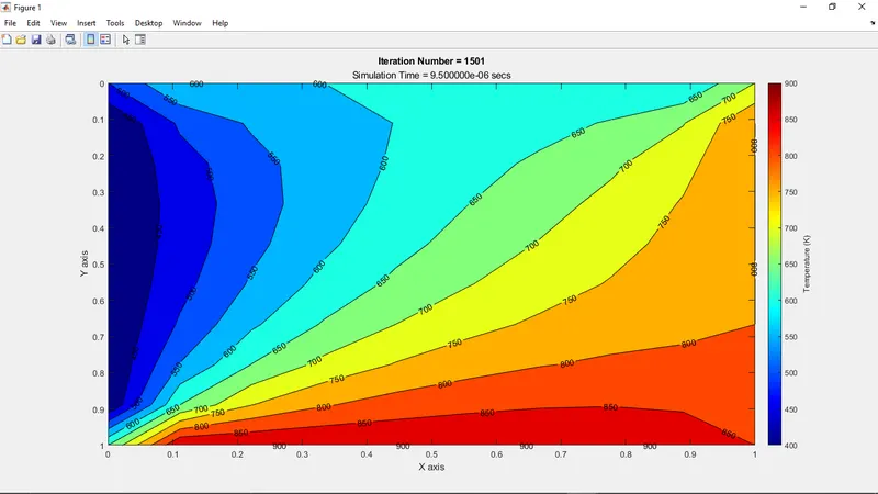
From the above plot we can see that it took 1501 iterations to have a steady solution.
Formula to calculate by Implicit Scheme:
Applying Forward Differencing to the Time Derivative terms and Central Differencing to the Spatial Terms
`(T_P^(n+1) - T_P^n)/dt = alpha*((T_R - 2*T_P + T_L)/dx^2+((T_T - 2*T_P + T_B)/(dy^2))^(n+1)`
`T_P^(n+1) =T_P^n+ dt*alpha*(((T_R - 2*T_P + T_L)/dx^2)+((T_T - 2*T_P + T_B)/(dy^2)))^(n+1)`
Taking all the (n+1) terms to one side and then solving we get
`T_P^(n+1) = 1/(1+2*k1+2*k2)*(T_P^n + k1*(T_L + T_R)^(n+1) + k2*(T_B + T_T)^(n+1))`
Where
`k1 = alpha*(dt/dx^2)`
`k2 = alpha*(dt/dy^2)`
Here k1 and k2 are the CFL numbers and also
The total value of CFL number must be less than equal to 0.5
i.e `CFL_T <= 0.5`
i.e `CFL_x + CFL_y <= 0.5`
We are calculating the value of T at (n+1) time node by using the values of T at 'n+1' node.
So here we have 1 known value and rest are unknown values, So for this scheme we will be using various Iterative Methods to calculate the values of T at (n+1) node.
MATLAB PROGRAM TO EVALUATE USING VARIOUS ITERATIVE METHODS:
% Transient State Analysis for 2D Heat Conduction

% Implicit Method

clear all
close all
clc

% Domain Length
L_x = 1;
L_y = L_x;

% Number of Nodes
nx = 10;
ny = nx;

x = linspace(0,1,nx);
y = linspace(0,1,ny);

dx = L_x/(nx-1);
%dx_1 = x(2)-x(1);

dy = L_y/(ny-1);
%dy_1 = y(2)-y(1);

T = 300*ones(nx,ny);

% Boundary Conditions
T(1,:) = 600;
T(:,1) = 400;
T(:,end) = 800;
T(end,:) = 900;

% Corner Conditions
T(1,1) = 500;
T(1,end) = 700;
T(end,1) = 650;
T(end,end) = 850;

Told = T;
T_prev = T;

error = 10e10;

tol = 1e-4;

dt = 0.001;

alpha = 1.4;

k1 = alpha*(dt/dx^2);
k2 = alpha*(dt/dy^2);

prompt = ('Enter the Solver Required ')
iterative_solver = input(prompt);


% Jacobi Solver

if iterative_solver==1
    j_iter = 1;

tic

% Time Loop
for t=1:1400

 % Convergence Loop
    while(error>tol)

    % Space Loop
    for i=2:nx-1
        for j=2:ny-1

            term_1 = 1/(1 + (2*k1) + (2*k2));
            term_2 = k1*term_1;
            term_3 = k2*term_1;
            H = (Told(i-1,j) + Told(i+1,j));
            V = (Told(i,j-1) + Told(i,j+1));

            T(i,j) = ((term_1*T_prev(i,j)) + (H*term_2) + (V*term_3));


        end
    end

        error = max(max(abs(Told-T)));
        Told = T;
        j_iter = j_iter + 1;

    end

    T_prev=T;

   error = 10e10;

end
 time_1=toc;

        figure(1)

    contourf(x,y,T,'ShowText','on')
    c = colorbar;
    c.Label.String = 'Temperature (K)'
    set(gca,'YDIR','reverse')
    colormap(jet)
    title_text=sprintf('Iteration Number = %d',j_iter);
    xlabel('X axis')
    ylabel('Y axis')
     s_t = sprintf('Simulation Time = %d secs',time_1);
    title(title_text,s_t)

end


% Gauss Siedal Solver

if iterative_solver==2
    gs_iter = 1;

tic

% Time Loop
for t=1:1400

 % Convergence Loop
    while(error>tol)

    % Space Loop
    for i=2:nx-1
        for j=2:ny-1

            term_1 = 1/(1 + (2*k1) + (2*k2));
            term_2 = k1*term_1;
            term_3 = k2*term_1;
            H = (T(i-1,j) + T(i+1,j));
            V = (T(i,j-1) + T(i,j+1));

            T(i,j) = ((term_1*T_prev(i,j)) + (H*term_2) + (V*term_3));


        end
    end

        error = max(max(abs(Told-T)));
        Told = T;
        gs_iter = gs_iter + 1;

    end

    T_prev=T;

   error = 10e10;

end
 time_2=toc;

        figure(2)

    contourf(x,y,T,'ShowText','on')
    c = colorbar;
    c.Label.String = 'Temperature (K)'
    set(gca,'YDIR','reverse')
    colormap(jet)
    title_text=sprintf('Iteration Number = %d',gs_iter);
    xlabel('X axis')
    ylabel('Y axis')
     s_t = sprintf('Simulation Time = %d secs',time_2);
    title(title_text,s_t)

end


% SOR Solver

omega = 1.2;

if iterative_solver==3
    sor_iter = 1;

tic

% Time Loop
for t=1:1400

 % Convergence Loop
    while(error>tol)

    % Space Loop
    for i=2:nx-1
        for j=2:ny-1

            term_1 = 1/(1 + (2*k1) + (2*k2));
            term_2 = k1*term_1;
            term_3 = k2*term_1;
            H = (T(i-1,j) + T(i+1,j));
            V = (T(i,j-1) + T(i,j+1));

            T(i,j) = ((term_1*T_prev(i,j)) + (H*term_2) + (V*term_3));
            T(i,j) = (1-omega)*Told(i,j) + omega*(T(i,j));


        end
    end

        error = max(max(abs(Told-T)));
        Told = T;
        sor_iter = sor_iter + 1;

    end

    T_prev=T;

   error = 10e10;

end
 time_3=toc;

        figure(3)

    contourf(x,y,T,'ShowText','on')
    c = colorbar;
    c.Label.String = 'Temperature (K)'
    set(gca,'YDIR','reverse')
    colormap(jet)
    title_text=sprintf('Iteration Number = %d',sor_iter);
    xlabel('X axis')
    ylabel('Y axis')
     s_t = sprintf('Simulation Time = %d secs',time_3);
    title(title_text,s_t)

end
Here in the above program we have defined a variable named 'T_prev' which stores the value of T at 'n' node and it shouldnot be updated inside the Convergence Loop but also it must be updated inside the Time Loop as for every space loop the old value of T i.e at n node must be a constant but for time loop it must get updated.
As we are using Iterative methods so there will be a Convergence loop to satisfy our error criteria and Time loop to evaluate for Temperature value at (n+1) time node.
The convergence loop must be inside the Time loop and both the for loops must be inside the Convergence Loop.
As per the requirement we have defined the values of k1,k2 and alpha and as per the hint given in the question we have formulated different terms.
Also we have to initialize the error value at starting of Time loop so that it takes the fresh value to calculate for new Time Interval.
For SOR method we need to define the value of 'Omega' which we have kept between 1.1 to 1.2 in order to Over Relax the solution to get faster result or less Iteration than Jacobi ans Gauss Siedal method.
For SOR Method we have used the formula
T(i,j) = (1 - omega)*Told(i,j) + omega*(T(Gauss Siedel Method) / T(Jacobi Method))
Here the Value of omega should be 1.1 or 1.2
PLOTS:
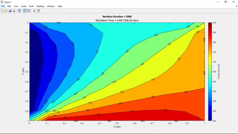
JACOBI METHOD:
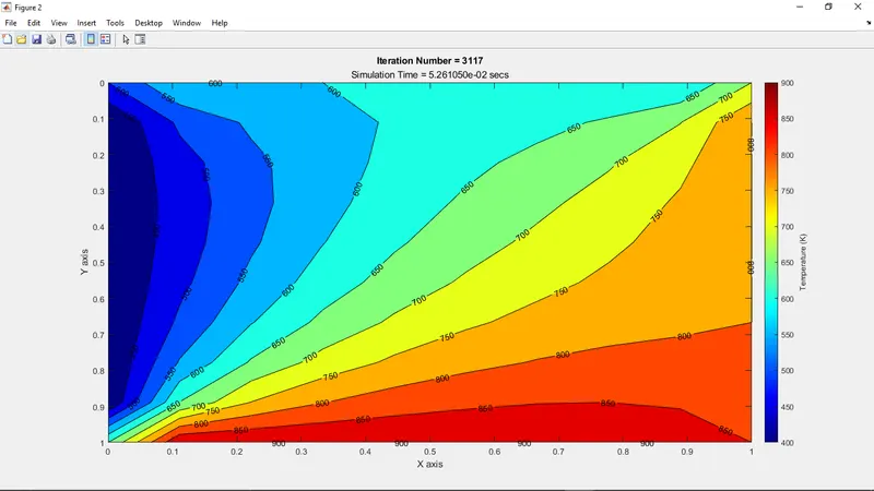
GAUSS SIEDEL METHOD:
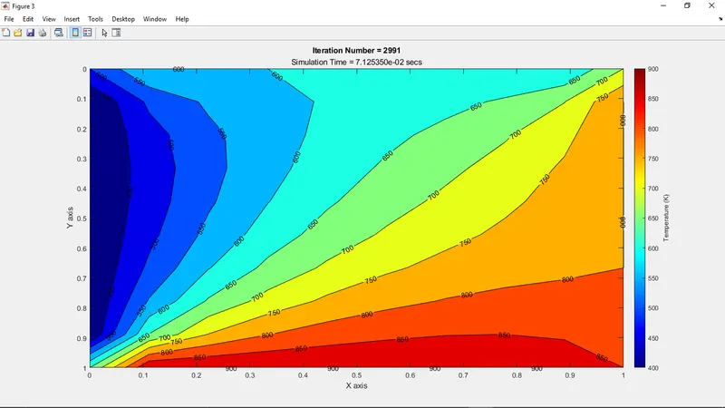
SOR METHOD:
CONCLUSION:
From the above contour plots we can conclude that all the three methods have achieved the steady state but Jacobi Method has taken more number of Iterations than Gauss Siedel Method and SOR Method and Gauss Siedel Method has taken more number of Iterations than SOR method.
Number of Iterations= Jacobi(3666) > Gauss Siedel(3117) > SOR(2991)