Week 7 - Simulation of a 1D Super-sonic nozzle flow simulation using Macormack Method
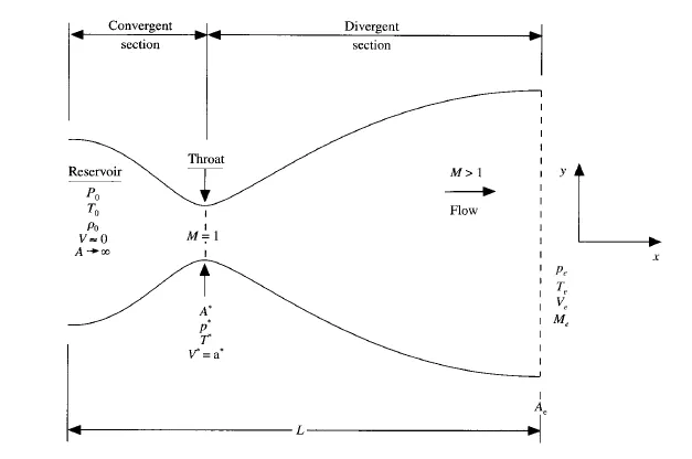
In the above problem we will be dealing with a Convergent Divergent Nozzle. As the flow to the inlet of the nozzle comes from a reservoir whose cross-sectional area is large hence the velocity of the flow is very small so the Mach number is less than 1 which says that the speed is subsonic.
Then the flow expands isentropically inside the nozzle to supersonic speed at the exit of the nozzle. The flow is basically subsonic at the convergent section to sonic at the throat and supersonic at the divergent section of the nozzle.
At the throat Mach number is equal to 1 which says that the local velocity of the flow is equal to the local speed of sound.
The flow properties are uniform along the cross section of the nozzle.
Although the area of the nozzle changes as a function of distance along the nozzle, x and therefore in reality the flow field is a two-dimensional i.e. the flow varies in the two-dimensional xy space, we make the assumption that the flow properties vary only with x, this flow is defined as Quasi-one-dimensional flow.
CFD SOLUTION OF SUBSONIC SUPERSONIC ISENTROPIC NOZZLE FLOW USING MACCORMACK'S METHOD:
GOVERNING EQUATIONS:
1. NON CONSERVATIVE FORM:
CONTINUITY EQUATION:
`(partialp')/(partialt') = -rho'*(partialv')/(partialx') - rho'*v'*(partial (lnA'))/(partialx') - v'*(partialrho')/(partialx')`
MOMENTUM EQUATION:
`(partialv')/(partialt') = -v'*(partialv')/(partialx') - 1/gamma*[(partialT')/(partialx') + (T')/(rho')*(partialrho')/(partialx'))]`
ENERGY EQUATION:
`(partialT')/(partialt') = -v'*(partialT')/(partialx') - (gamma-1)*T'*[(partialv')/(partialx') + v'*(partialln(A'))/(partialx')]`
2. CONSERVATIVE FORM:
CONTINUITY EQUATION:
`(partial (rho'*A'))/(partialt') + (partial (rho'*A'*v'))/(partialx') = 0`
MOMENTUM EQUATION:
`(partial (rho'*A'*v'))/(partialt') + (partial [(rho'*A'*v'^2) + (1/gamma)*p'*A'])/(partialx') = (1/gamma)*p'*(partialA')/(partialx')`
ENERGY EQUATION:
`(partial([ rho'*((e')/(gamma-1) + (gamma/2)v'^2)*A' ]))/(partialt') + (partial([rho'*((e')/(gamma-1) + (gamma/2)v'^2)*v'*A' + p'*A'*v']))/(partialx') = 0`
where
T' = Non Dimensional Temperature = `T/T_0`
`rho' =`Non Dimensional Density = `rho/rho_0`
L = Length of the Nozzle
x' = Dimensionless Length of the Nozzle = x/L
`a_0`= Speed of Sound in Reservoir = `sqrt(gamma*R*T)`
v' = Dimensionless Velocity = `v/a_0`
t' = Dimensionless Time = `t/(L/a_0)`
A' = Dimensionless Area = `A/A^**`
`A^**`= Area at the throat of the Nozzle or Sonic Area
SOLVING THE ABOVE METHOD USING MACCORMACK'S METHOD:
MACCORMACK'S METHOD:
Maccormack's Method is a variant of Lax-Wendroff approach but is much simpler in its application. It is an Explicit-Finite difference method which is second order accurate in both space and time.
This method is basically divided into 2 Stages:
1. Predictor Step:
Here we find the derivative of variables with respect to time by forward differencing of space terms.
Then we update the solution of the variables by using the initial value.
2. Corrector Step:
Here we find the derivative of the variables with respect to time by backward differencing of space terms.
After completing both the prdictor and corrector step the actual value of time derivative is calculated by taking the average of both these terms
And the final solution of the variable is updated by using the old/Initial value.
Solving the Non Conservative form:
Initial Conditions:
`rho = 1 - 0.3146*x`
`T = 1 - 0.2314*x`
`v = (0.1 + 1.09*x)*T^(1/2)`
`A = 1 + 2.2*(x - 1.5)^2` for `0<=x<=3`
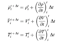
1. Predictor Step
Continuity Equation

Momentum Equation

Energy Equation

Intermediate Solution Update
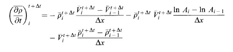
2. Corrector Step
Continuity Equation
Momentum Equation

Energy Equation
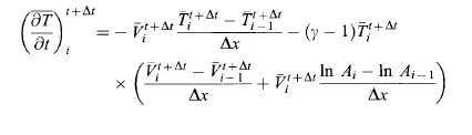
Average of Predictor and Corrector Step:
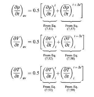
Final Solution Update
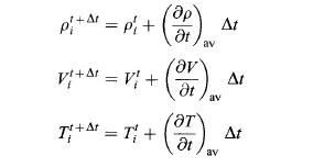
CALCULATION OF TIME STEP:
`deltat = min(c*((deltax)/(a+v)))`
where
c = Courant Number
dx = space between the nodes
a = Speed of Sound
V = Local velocity of flow
BOUNDARY CONDITIONS:
Since we are assuming that flow only occurs in the x direction so at the inlet we should provide one value to float and keep other values to be constant and at the outlet as the flow changes from subsonic to sonic to supersonic and exits out of the nozzle we must define all the values.
The inlet and outlet boundary conditions are calculated using linear extrapolation method.
At Inlet
1. `v_1 = 2*v_2 -v_3`
At Outlet
1. `v_n = 2*v_(n-1) - v_(n-2)`
2. `rho_n = 2*rho_(n-1)-rho_(n-2)`
3. `T_n = 2*T_(n-1)-T_(n-2)`
where n is the last node.
Solving the Conservative form:
The Continuity, Momentum, Energy equations in Conservative form can be expressed in a generic form.
Let us define the elements of the solution vector U, the flux vector F and the source term J as follows:
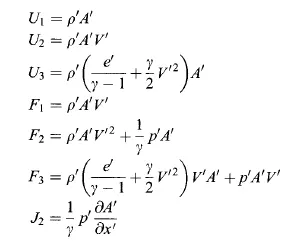
Using the above values our equations become
1. Continuity Equation
`(partialU_1)/(partialt') = -(partialF_1)/(partialx')`
2. Momentum Equation
`(partialU_2)/(partialt') = -(partialF_2)/(partialx') +J_2`
3. Energy Equation
`(partialU_3)/(partialt') = -(partialF_3)/(partialx')`
FLOW VARIABLES:
1.`rho' = U_1/(A')`
2.`v' = U_2/U_1`
3. `T'=e'=(gamma-1)*((U_3/U_1) - (gamma/2)*v'^2)`
4. `p'=rho'*T'`
PURE FORM OF FLUX TERMS
The flux terms are the functions of U and therefore they can be written in terms of U as follows:
1.`F_1=U_2`
2. `F_2 = U_2^2/U_1 +(gamma-1)/gamma*(U_3-(gamma/2)*U_2^2/U_1)`
3. `F_3 = gamma*(U_2*U_3)/U_1 - gamma*(gamma-1)/2*U_2^3/U_1^2`
4. `J_2 = (gamma-1)/gamma*(U_3-(gamma/2)*U_2^2/U_1)*(partialln(A'))/(partialx')`
Initial Conditions:
for `0<=x<=0.5`
`rho'=1.0`
`T'=1.0`
for `0.5<=x<=1.5`
`rho'=1.0-0.366*(x-0.5)`
`T'=1.0-0.167*(x-0.5)`
for `1.5<=x<=3.5`
`rho'=0.634-0.3879*(x-1.5)`
`T'=0.833-0.3507*(x-1.5)`
`v'=0.59/(rho'*A')`
`U_1=rho'*A'`
`U_2=rho'*A'*v'`
`U_3=rho'*(((T')/(gamma-1)) + gamma/2*v'^2)*A'`
Time Step Calculation:
`deltat = min(c*((deltax)/(a+v)))`
where
c = Courant Number
dx = space between the nodes
a = Speed of Sound
V = Local velocity of flow
1.Predictor Step:
1.`(dF1)/dx = (F1(i+1) - F1(i))/dx;`
2.`(dF2)/dx = (F2(i+1) - F2(i))/dx;`
3.`(dF3)/dx = (F3(i+1) - F3(i))/dx;`
1. Continuity Equation
`(partialU_1)/(partialt') = -(partialF_1)/(partialx')`
2. Momentum Equation
`(partialU_2)/(partialt') = -(partialF_2)/(partialx') +J_2`
3. Energy Equation
`(partialU_3)/(partialt') = -(partialF_3)/(partialx')`
Intermediate Solution Update:
`U_1(i) = U_1old(i) + (dU_1)/dt*dt`
`U_2(i) = U_2old(i) + (dU_2)/dt*dt`
`U_3(i) = U_3old(i) + (dU_3)/dt*dt`
2.Corrector Method:
1. `(dF1)/dx = (F1(i) - F1(i-1))/dx`
2.`(dF2)/dx = (F2(i) - F2(i-1))/dx;`
3.`(dF3)/dx = (F3(i) - F3(i-1))/dx;`
1. Continuity Equation
`(partialU_1)/(partialt') = -(partialF_1)/(partialx')`
2. Momentum Equation
`(partialU_2)/(partialt') = -(partialF_2)/(partialx') +J_2`
3. Energy Equation
`(partialU_3)/(partialt') = -(partialF_3)/(partialx')`
Average of Predictor and Corrector Step
1. `(dU_1)/dt = 0.5*((dU_1)/dt)_p + ((dU_1)/dt)_c`
2. `(dU_2)/dt = 0.5*((dU_2)/dt)_p + ((dU_2)/dt)_c`
3. `(dU_3)/dt = 0.5*((dU_3)/dt)_p + ((dU_3)/dt)_c`
Solution Update:
`U_1(i) = U_1old(i) + ((dU_1)/dt)_(avg)*dt`
`U_2(i) = U_2old(i) + ((dU_2)/dt)_(avg)*dt`
`U_3(i) = U_3old(i) + ((dU_3)/dt)_(avg)*dt`
Boundary Conditions:
At Inlet:
`U_1(1) = rho(1)*A(1)`
`U_2(1) = 2*U_2(2) - U_2(3)`
`U_3(1) = U_1(1)*((T(1))/(gamma - 1) + gamma/2*v(1)^2)`
At Outlet:
`U_1(n) = 2*U_1(n-1) - U_1(n-2)`
`U_2(n) = 2*U_2(n-1) - U_2(n-2)`
`U_3(n) = 2*U_3(n-1) - U_3(n-2)`
MATLAB CODE TO EVALUATE THE ABOVE PROBLEM:
FUNCTION FOR NON CONSERVATIVE METHOD
function [rho_nc , rho_th , T_nc , T_th , v_nc , v_th , mdot_nc , mdot_th , M_nc , M_th , P_nc , P_th] = non_conservative(n,x,dx,nt,A,gamma,c,throat)

rho = 1 - 0.3146*x;
T = 1 - 0.2314*x;
v = (0.1 + 1.09*x).*T.^(0.5);
dt = min((c*dx)./((sqrt(T)) + v));

% Outer Time loop

for k = 1:nt

    rho_old = rho;
    T_old = T;
    v_old = v;

    % Predictor Method

    for i = 2:n-1

        dvdx = (v(i+1) - v(i))/dx;
        drhodx = (rho(i+1) - rho(i))/dx;
        dTdx = (T(i+1) - T(i))/dx;
        dlogAdx = (log(A(i+1)) - log(A(i)))/dx;

        % Continuity Equation

        drhodt_p(i) = -rho(i)*dvdx - rho(i)*v(i)*dlogAdx - v(i)*drhodx;

        % Momentum Equation

        dvdt_p(i) = -v(i)*dvdx - (dTdx + (T(i)/rho(i))*drhodx)/gamma;

        % Energy Equation

        dTdt_p(i) = -v(i)*dTdx - (gamma - 1)*T(i)*(dvdx + v(i)*dlogAdx);

        % Solution Update
        rho(i) = rho_old(i) + drhodt_p(i)*dt;
        v(i) = v_old(i) + dvdt_p(i)*dt;
        T(i) = T_old(i) + dTdt_p(i)*dt;

    end

    % Corrector Method


    for i = 2:n-1

        dvdx = (v(i) - v(i-1))/dx;
        drhodx = (rho(i) - rho(i-1))/dx;
        dTdx = (T(i) - T(i-1))/dx;
        dlogAdx = (log(A(i)) - log(A(i-1)))/dx;

        % Continuity Equation

        drhodt_c(i) = -rho(i)*dvdx - rho(i)*v(i)*dlogAdx - v(i)*drhodx;

        % Momentum Equation

        dvdt_c(i) = -v(i)*dvdx - (dTdx + (T(i)/rho(i))*drhodx)/gamma;

        % Energy Equation

        dTdt_c(i) = -v(i)*dTdx - (gamma - 1)*T(i)*(dvdx + v(i)*dlogAdx);


    end

    % Computing the Average

    drhodt = 0.5*(drhodt_p + drhodt_c);
    dvdt = 0.5*(dvdt_p + dvdt_c);
    dTdt = 0.5*(dTdt_p + dTdt_c);

    for i = 2:n-1

        rho(i) = rho_old(i) + drhodt(i)*dt;
        v(i) = v_old(i) + dvdt(i)*dt;
        T(i) = T_old(i) + dTdt(i)*dt;

    end

     mdot = rho.*A.*v;
     M = v./sqrt(T);
     P = rho.*T;
     rho_th(k) = rho(throat);
     v_th(k) = v(throat);
     T_th(k) = T(throat);
     mdot_th(k) = mdot(throat);
     M_th(k) = M(throat);
     P_th(k) = P(throat);

    % Applying Boundary Conditions
    % Inlet
    v(1) = 2*v(2) - v(3);

    % Outlet
    v(n) = 2*v(n-1) - v(n-2);
    rho(n) = 2*rho(n-1) - rho(n-2);
    T(n) = 2*T(n-1) - T(n-2);

%     plot(x,v)
%     title(sprintf('Time Step = %d',k))
%     pause(0.03)

        figure(1)

    if k==25
        plot(x,mdot,'r','linewidth',1.5)
        hold on
    elseif k==50
        plot(x,mdot,'g','linewidth',1.5)
        hold on
    elseif k==100
        plot(x,mdot,'b','linewidth',1.5)
        hold on
    elseif k==200
        plot(x,mdot,'c','linewidth',1.5)
        hold on
    elseif k==400
        plot(x,mdot,'m','linewidth',1.5)
        hold on
    elseif k==800
        plot(x,mdot,'y','linewidth',1.5)
        hold on
    elseif k==1400
        plot(x,mdot,'k','linewidth',1.5)

        xlabel('Nozzle Length')
        ylabel('Mass Flow Rate')
        legend('25','50','100','200','400','800','1400')
        title('Nozzle Length vs Mass flow rate in Non Conservative Form')
    end


end

rho_nc = rho;
T_nc = T;
v_nc = v;
mdot_nc = mdot;
M_nc = M;
P_nc = P;


end
FUNCTION FOR CONSERVATIVE METHOD
function [rho_c , rho_th2 , T_c , T_th2 , v_c , v_th2 , mdot_c , mdot_th2 , M_c , M_th2 , P_c , P_th2] = conservative(n,x,dx,nt,A,gamma,c,throat)


% Initial Properties

for i=1:n

if (x(i) >= 0 && x(i) <= 0.5)
    rho(i) = 1;
    T(i) = 1;

elseif (x(i) >= 0.5 && x(i) <= 1.5)
    rho(i) = 1 - 0.366*(x(i) - 0.5);
    T(i) = 1 - 0.167*(x(i) - 0.5);

else
    rho(i) = 0.634 - 0.3879*(x(i) - 1.5);
    T(i) = 0.833 - 0.3507*(x(i) - 1.5);

end
end

P = rho.*T;
v = 0.59./(rho.*A);
mdot = rho.*A.*v;

% % calculating dt
dt = min((c*dx)./((sqrt(T)) + v));

rho_old = rho;
T_old = T;
v_old = v;

nt = 1400;
% dt = 0.0267;

% Solution Variable Initialization

U1 = rho.*A;
U2 = U1.*v;
U3 = rho.*A.*((T/(gamma-1)) + 0.5.*gamma.*v.^2);

for k = 1:nt

    U1_old = U1;
    U2_old = U2;
    U3_old = U3;

    % Initialization of Flux

    F1 = U2;
    F2 = (U2.^2)./U1 + ((gamma-1)/gamma).*(U3 - 0.5.*gamma.*(U2.^2)./U1);
    F3 = gamma.*((U2.*U3)./U1) - (gamma.*0.5.*(gamma-1).*(U2.^3./U1.^2));

    % Predictor Method

    for i = 2:n-1

        dlogAdx(i) = (log(A(i+1)) - log(A(i)))/dx;
        dAdx = (A(i+1) - A(i))/dx;

        J2(i) = (1/gamma)*rho(i)*T(i)*dAdx;

        dF1dx = (F1(i+1) - F1(i))/dx;
        dF2dx = (F2(i+1) - F2(i))/dx;
        dF3dx = (F3(i+1) - F3(i))/dx;

        % Continuity Equation

        dU1dt_p(i) = -dF1dx;

        % Momentum Equation

        dU2dt_p(i) = -dF2dx + J2(i);

        % Energy Equation

        dU3dt_p(i) = -dF3dx;


        % Solution Update

        U1(i) = U1_old(i) + dU1dt_p(i)*dt;
        U2(i) = U2_old(i) + dU2dt_p(i)*dt;
        U3(i) = U3_old(i) + dU3dt_p(i)*dt;

    end

        % Initialization of Flux

    F1 = U2;
    F2 = (U2.^2)./U1 + ((gamma-1)/gamma).*(U3 - 0.5.*gamma.*(U2.^2)./U1);
    F3 = gamma.*((U2.*U3)./U1) - (gamma.*0.5.*(gamma-1).*(U2.^3./U1.^2));

        % Corrector Method

    for i = 2:n-1

        dlogAdx(i) = (log(A(i)) - log(A(i-1)))/dx;
        dAdx = (A(i) - A(i-1))/dx;

        J2(i) = (1/gamma)*rho(i)*T(i)*dAdx;
        dF1dx = (F1(i) - F1(i-1))/dx;
        dF2dx = (F2(i) - F2(i-1))/dx;
        dF3dx = (F3(i) - F3(i-1))/dx;

        % Continuity Equation

        dU1dt_c(i) = -dF1dx;

        % Momentum Equation

        dU2dt_c(i) = -dF2dx + J2(i);

        % Energy Equation

        dU3dt_c(i) = -dF3dx;


    end

    % Computing the Average

    dU1dt = 0.5*(dU1dt_p + dU1dt_c);
    dU2dt = 0.5*(dU2dt_p + dU2dt_c);
    dU3dt = 0.5*(dU3dt_p + dU3dt_c);

    for i = 2:n-1

        U1(i) = U1_old(i) + dU1dt(i)*dt;
        U2(i) = U2_old(i) + dU2dt(i)*dt;
        U3(i) = U3_old(i) + dU3dt(i)*dt;

    end

    % Applying Boundary Conditions
    % Inlet Subsonic Inflow

    U1(1) = rho(1)*A(1);
    U2(1) = 2*U2(2) - U2(3);
    U3(1) = U1(1)*(T(1)/(gamma - 1) + 0.5*gamma*v(1)^2);

    % Outlet Supersonic Outflow

    U1(n) = 2*U1(n-1) - U1(n-2);
    U2(n) = 2*U2(n-1) - U2(n-2);
    U3(n) = 2*U3(n-1) - U3(n-2);


   % Updating Flow Variables
   rho = U1./A;
   v = U2./U1;
   T = (gamma - 1).*((U3./U1) - 0.5.*gamma.*v.^2);
   P = rho.*T;
   mdot = rho.*A.*v;
   M = v./sqrt(T);

     rho_th2(k) = rho(throat);
     v_th2(k) = v(throat);
     T_th2(k) = T(throat);
     mdot_th2(k) = mdot(throat);
     M_th2(k) = M(throat);
     P_th2(k) = P(throat);

%     plot(x,v)
%     title(sprintf('Time Step = %d',k))
%     pause(0.03)


      figure(2)

    if k==25
        plot(x,mdot,'r','linewidth',1.5)
        hold on
    elseif k==50
        plot(x,mdot,'g','linewidth',1.5)
        hold on
    elseif k==100
        plot(x,mdot,'b','linewidth',1.5)
        hold on
    elseif k==200
        plot(x,mdot,'c','linewidth',1.5)
        hold on
    elseif k==400
        plot(x,mdot,'m','linewidth',1.5)
        hold on
    elseif k==800
        plot(x,mdot,'y','linewidth',1.5)
        hold on
    elseif k==1400
        plot(x,mdot,'k','linewidth',1.5)

        xlabel('Nozzle Length')
        ylabel('Mass Flow Rate')
        legend('25','50','100','200','400','800','1400')
        title('Nozzle Length vs Mass flow rate in Conservative Form')

    end

rho_c = rho;
T_c = T;
v_c = v;
mdot_c = mdot;
M_c = M;
P_c = P;


end
MAIN PROGRAM:
clear all
close all
clc

n = 91;
x = linspace(0,3,n);
dx = x(2)-x(1);
c = 0.5;
throat = (n+1)/2;
gamma = 1.4;
A = 1 + 2.2.*(x - 1.5).^2;
nt = 1400;
ts = [1:1400];
% dt = 0.0267;


% NON CONSERVATIVE FORM
[rho_nc , rho_th , T_nc , T_th , v_nc , v_th , mdot_nc , mdot_th , M_nc , M_th , P_nc , P_th] = non_conservative(n,x,dx,nt,A,gamma,c,throat);

% CONSERVATIVE FORM
[rho_c , rho_th2 , T_c , T_th2 , v_c , v_th2 , mdot_c , mdot_th2 , M_c , M_th2 , P_c , P_th2] = conservative(n,x,dx,nt,A,gamma,c,throat);


    figure(3)
    sgtitle('Nozzle Length vs Dimensionless Flow Variables in Both Forms')

    subplot(4,1,1)
    plot(x,rho_nc)
    hold on
    plot(x,rho_c,'o')
    xlim([0 3])
    xlabel('Nozzle Length')
    ylabel('Density Ratio')
    legend('Non Conservative','Conservative')

    subplot(4,1,2)
    plot(x,T_nc)
    hold on
    plot(x,T_c,'o')
    xlim([0 3])
    xlabel('Nozzle Length')
    ylabel('Temperature Ratio')

    subplot(4,1,3)
    plot(x,M_nc)
    hold on
    plot(x,M_c,'o')
    xlim([0 3])
    xlabel('Nozzle Length')
    ylabel('Mach Number')

    subplot(4,1,4)
    plot(x,P_nc)
    hold on
    plot(x,P_c,'o')
    xlim([0 3])
    xlabel('Nozzle Length')
    ylabel('Pressure Ratio')


    figure(4)
    sgtitle('Time Steps vs Dimensionless Flow Variables at throat in both Forms')

    subplot(4,1,1)
    plot(ts,rho_th)
    hold on
    plot(ts,rho_th2)
    xlim([0 1400])
    xlabel('Time Steps')
    ylabel('Density Ratio')
    legend('Non Conservative','Conservative')

    subplot(4,1,2)
    plot(ts,T_th)
    hold on
    plot(ts,T_th2)
    xlim([0 1400])
    xlabel('Time Steps')
    ylabel('Temperature Ratio')

    subplot(4,1,3)
    plot(ts,M_th)
    hold on
    plot(ts,M_th2)
    xlim([0 1400])
    xlabel('Time Steps')
    ylabel('Mach Number')

    subplot(4,1,4)
    plot(ts,P_th)
    hold on
    plot(ts,P_th2)
    xlim([0 1400])
    xlabel('Time Steps')
    ylabel('Pressure Ratio')

    figure(5)

    plot(x,mdot_nc,'r','linewidth',1.5)
    hold on
    plot(x,mdot_c,'g','linewidth',1.5)
    xlabel('Nozzle Length')
    ylabel('Mass flow rate')
    legend('Non-Conservative','Conservative')
    title('Mass flow rate in both Non conservative and Conservative form')


    figure(6)
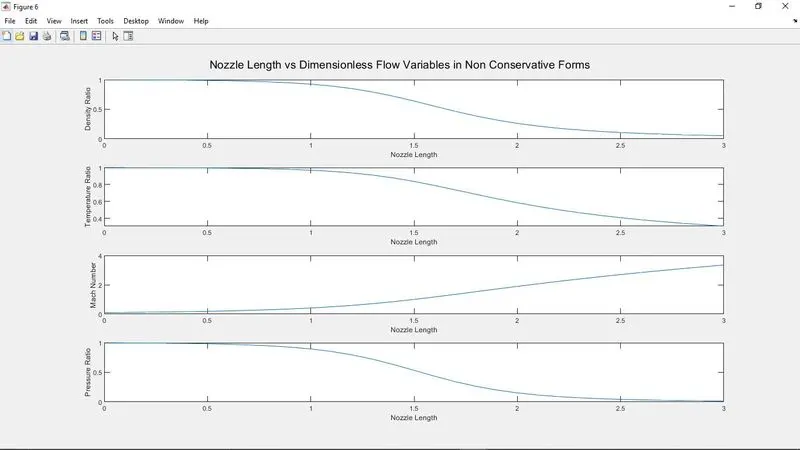
    sgtitle('Nozzle Length vs Dimensionless Flow Variables in Non Conservative Forms')

    subplot(4,1,1)
    plot(x,rho_nc)
    xlim([0 3])
    xlabel('Nozzle Length')
    ylabel('Density Ratio')

    subplot(4,1,2)
    plot(x,T_nc)
    xlim([0 3])
    xlabel('Nozzle Length')
    ylabel('Temperature Ratio')

    subplot(4,1,3)
    plot(x,M_nc)
    xlim([0 3])
    xlabel('Nozzle Length')
    ylabel('Mach Number')

    subplot(4,1,4)
    plot(x,P_nc)
    xlim([0 3])
    xlabel('Nozzle Length')
    ylabel('Pressure Ratio')


    figure(7)
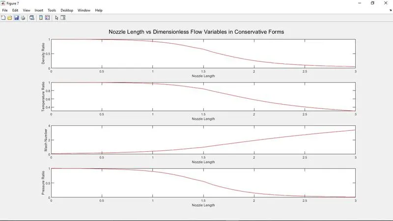
    sgtitle('Nozzle Length vs Dimensionless Flow Variables in Conservative Forms')

    subplot(4,1,1)
    plot(x,rho_c,'r')
    xlim([0 3])
    xlabel('Nozzle Length')
    ylabel('Density Ratio')

    subplot(4,1,2)
    plot(x,T_c,'r')
    xlim([0 3])
    xlabel('Nozzle Length')
    ylabel('Temperature Ratio')

    subplot(4,1,3)
    plot(x,M_c,'r')
    xlim([0 3])
    xlabel('Nozzle Length')
    ylabel('Mach Number')

    subplot(4,1,4)
    plot(x,P_c,'r')
    xlim([0 3])
    xlabel('Nozzle Length')
    ylabel('Pressure Ratio')
In the main program first we have defined the variables that are constant and coomon for both the conservative and non conservative forms.
We have calculated the point where throat section of the nozzle is present and defined the area of the nozzle.
Here we have specified the time steps as 1400 and we will be formulating the above problem with 3 different grids to understand the grid independency.
Then we have called our functions for both Conservative and Non conservative forms by giving required arguements that will be required to solve them, and also given respective variables to store the output as the reults of the function.
Inside the functions we have defined our flow variables that are Density, Temperature, Velocity and have calculated the time steps size by using the formula described above.
Then we have written the outer time loop so that it will calculate the flow variables for different time.
Inside the Time loop we have stored our variables in an other variable in order to use then at the final solution calculation.
Then we have written our Predictor steps as derived above then updated the values of flow variables so that it will be used in the corrector steps. After writting the corrector steps we have calculated the average between the predictor step and corrector step, and atlast we have updated our final solution to get the stable result of flow variables.
After that we have calculated our mass flow rate, Mach number and different values of our float variables at the throat of the nozzle.
At the end we have given our boundary conditions required to solve the problem.The boundary condition involves the Inlet condition and Outlet condition.
The same procedure is followed for both the forms.
After that we have plotted different types of graphs using the above solution.The plots are:
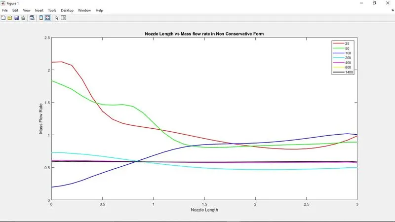
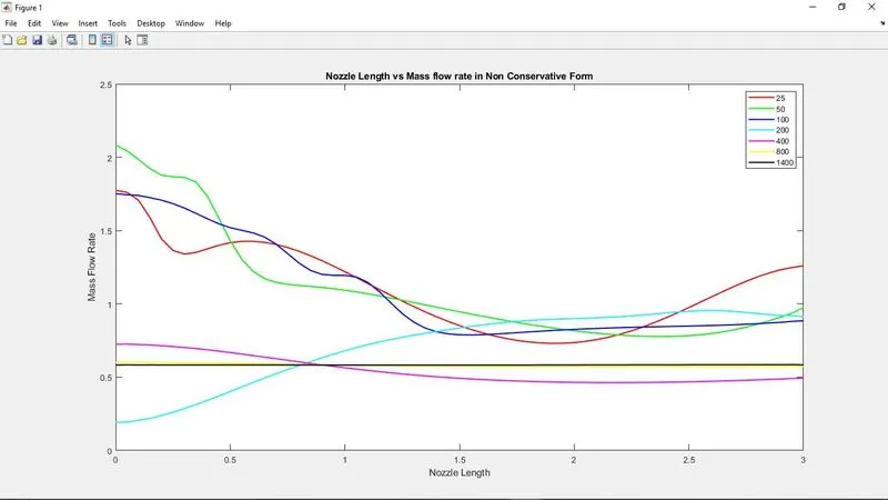
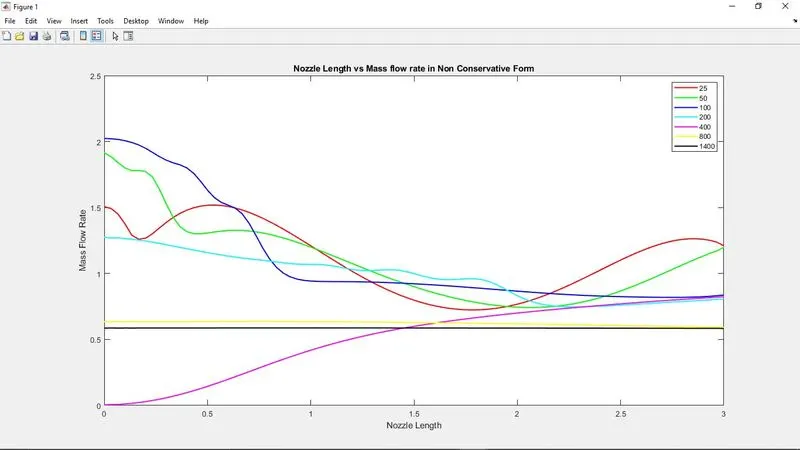
1. Nozzle Length vs Mass flow rate at different time steps for Non Conservative form
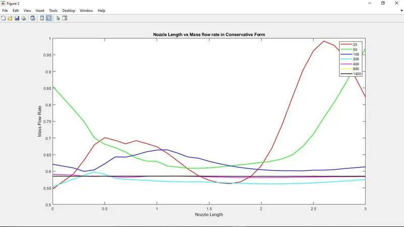
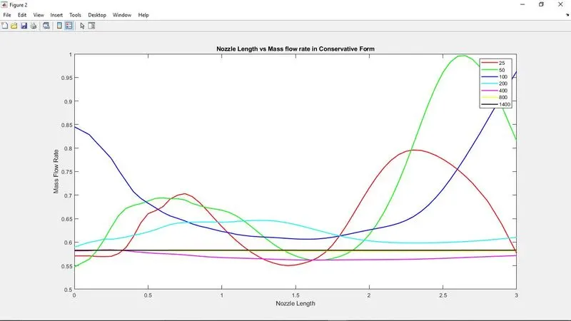
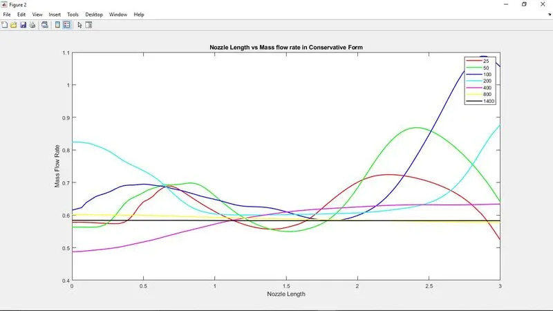
2. Nozzle Length vs Mass flow rate at different time steps for Conservative form
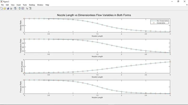
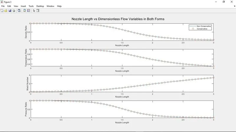
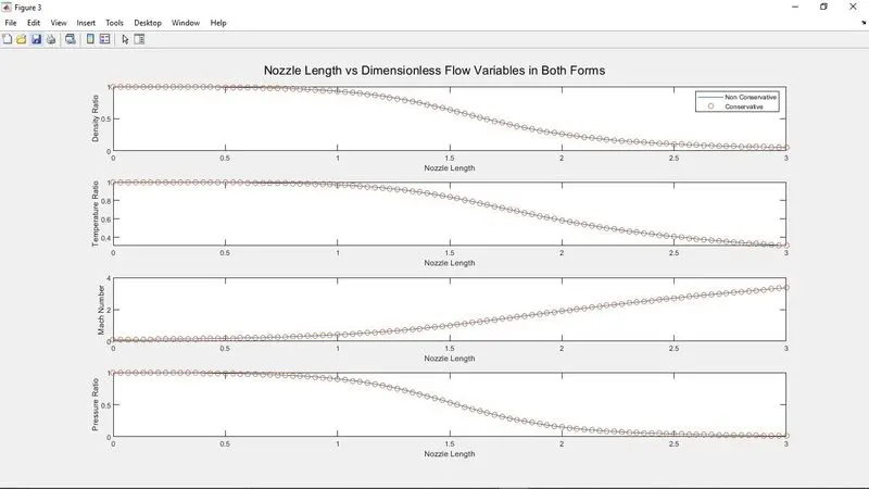
3. Nozzle length vs Dimensionless flow variables in both forms
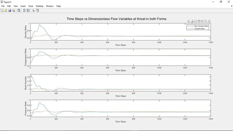
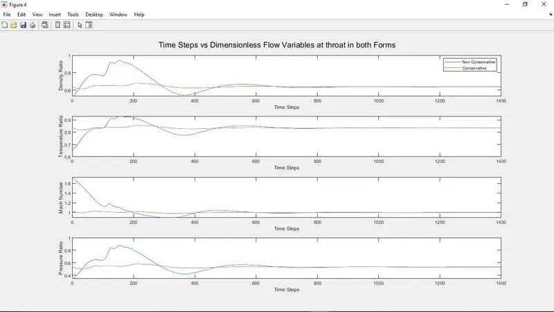
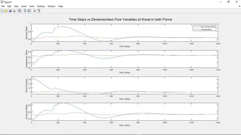
4. Time Steps vs Dimensionless Flow Variables at throat in both Forms
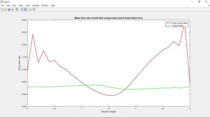
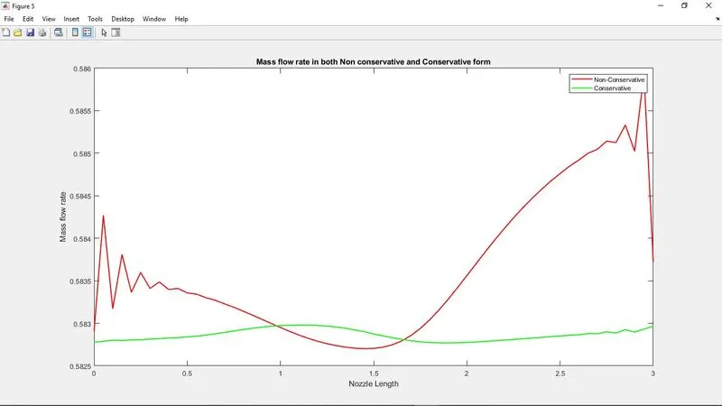
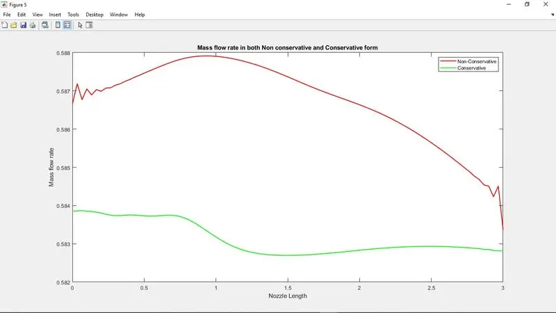
5. Comparision of Mass flow rate in both the forms.
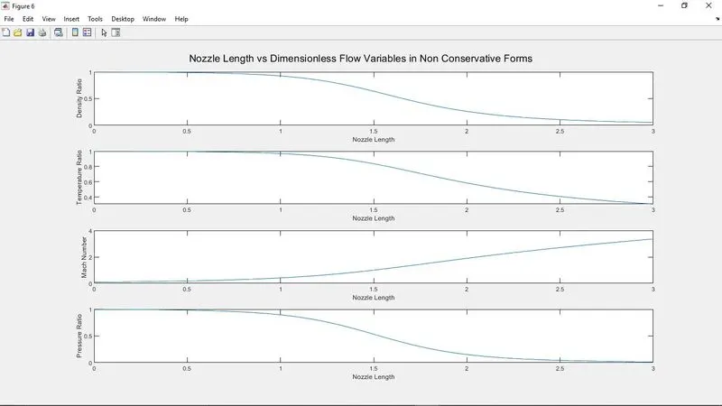
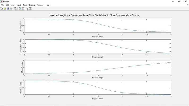
6. Nozzle Length vs Dimensionless Flow Variables in Non Conservative Forms
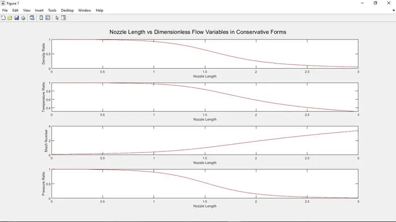
7. Nozzle Length vs Dimensionless Flow Variables in Conservative Forms
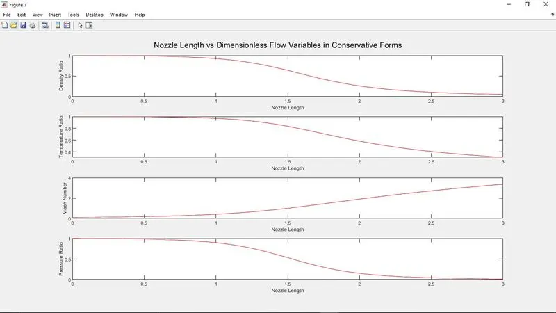
PLOTS:
AT 31 NODES/GRIDS:
AT 61 NODES/GRIDS:
AT 91 NODES/GRIDS:
GRID INDEPENDENCE TEST:
This test is conducted between the Analytical solution and the Numerical solution in order to check that if we increase our grid size then our solution gets changed or not.
If also by changing the grid size we obtain the same value of flow variables in all the conditions we can say that our solution is grid independent.
So here in this problem we have selected 31,61,91 as three different values of grid in order to check our grid independency and we have compared at the throat.
FOR 31 NODES:
| @31 Nodes | EXACT SOLUTION | NON CONSERVATIVE FORM | CONSERVATIVE FORM |
| `rho'` | 0.634 | 0.6387 | 0.6535 |
| `T'` | 0.833 | 0.8365 | 0.8416 |
| `P'` | 0.528 | 0.5342 | 0.5500 |
| M | 1 | 0.9994 | 0.9760 |
FOR 61 NODES:
| @61 Nodes | EXACT SOLUTION | NON CONSERVATIVE FORM | CONSERVATIVE FORM |
| `rho'` | 0.634 | 0.9691 | 0.9690 |
| `T'` | 0.833 | 0.9875 | 0.9875 |
| `P'` | 0.528 | 0.9570 | 0.9569 |
| M | 1 | 0.2706 | 0.2706 |
FOR 91 NODES:
| @91 Nodes | EXACT SOLUTION | NON CONSERVATIVE FORM | CONSERVATIVE FORM |
| `rho'` | 0.634 | 0.9899 | 0.9882 |
| `T'` | 0.833 | 0.9960 | 0.9952 |
| `P'` | 0.528 | 0.9859 | 0.9835 |
| M | 1 | 0.1850 | 0.1858 |
From the above tables it can be clearly seen that only for grid size of 31 the Numerical solution is very close to Analytical solution while for grid size 61 and 91 they are not near to close.
So it can be concluded that it is not grid independent.
CONCLUSION:
FIGURE 1:
In figure 1 we have plotted mass flow rate throughout the nozzle length at different time steps for Non conservative form.
And from the plot we can observe that for Time slots less than 400 the mass flow rate oscillates aggressively and the flow rate is not stable and after 400 Time steps it becomes almost straight line which means that mass flow rate became stable after 400 time steps.
FIGURE 2:
In figure 1 we have plotted mass flow rate throughout the nozzle length at different time steps for conservative form.
And from the plot we can observe that for Time slots less than 400 the mass flow rate oscillates aggressively and the flow rate is not stable and after 400 Time steps it becomes almost straight line which means that mass flow rate became stable after 400 time steps.
From the above two figures it can be concluded that as the Time Steps increases mass flow rate inside the nozzle becomes stable and after a particular time period it becomes a constant.
FIGURE 3:
In our third plot we have compared how the Non dimensional flow variables Density, Pressure, Temperature and Mach Number varies along the length of the nozzle for both Conservative and Non conservative form.
This graph was plotted to compare between the two forms and check if it matches with the analytical solution.
From the above it can be concluded that the values of non dimensional flow variables in both conservative and non conservative forms are same as both the plots coincides each other.
FIGURE 4:
In our fourth figure we have plotted how flow variables at the throat varies with different time steps, and we have plotted both the forms in it in order to compare between the two.
From the above it can be concluded that the flow variables at the throat in both forms becomes stable after 400 time steps.
Initially in Non conservative form the flow variables oscillated aggressively and after 200 steps it damps and after 400 steps it becomes constant while in conservative form at the initial stages it doesnot oscillate aggresively.
FIGURE 5:
In our fifth figure we have plotted how mass flow rate varies along the length of the nozzle for both the Non conservative and conservative forms.
From the above graph it can be clearly observed that in the Non conservative form mass flow rate oscillates or varies vigourously while in Conservative form it varies very little and remains almost constant.
FIGURE 6:
In figure 6 we have plotted how non dimensional flow variables vary along the length of the nozzle for Non conservative form, and it completely matches with our solution from our reference book.
FIGURE 7:
In figure 6 we have plotted how non dimensional flow variables vary along the length of the nozzle for conservative form, and it completely matches with our solution from our reference book.