2D Element Formulation for Beam

AIM:

• To obtain the result for the beam model using the default element formulation values and the recommended element formulation values.

OBJECTIVES OF THE PROJECT:

• To run the radios file to obtain the results for the beam section.
• To run the simulation for 55 millisecond.
• To run the simulation using the default element formulation values.
• To run the simulation using the recommended element formulation values.
• To obtain the von mises stress and deformation on the beam section.
• To understand the Hyperview window.
• To plot graphs with the results file in the Hypergraph window.
• To compare the energy error and mass error for the two case models.
• To understand the difference and the reason for reducing the energy error.

PROCEDURE:

• First step is to import the model into the Hypermesh radios solver profile.
• Go to FILE > IMPORT SOLVER DECK > BROWSE > OPEN > IMPORT.
• 
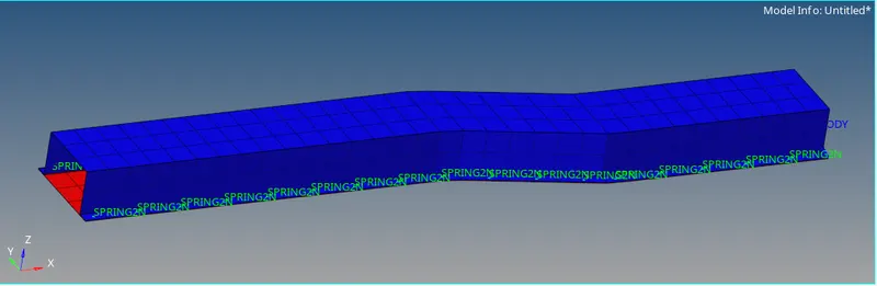
• Now the model will open in the GUI area.
• Go to the TAB AREA > CARDS > ENG_RUN > TSTOP = 55.
• 
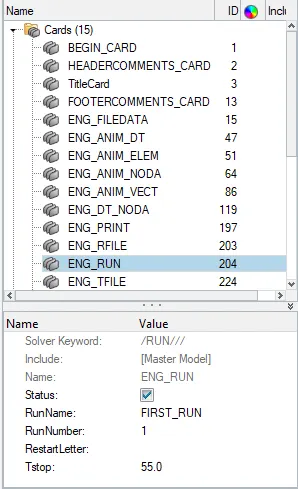
• This will set the run time to 55 ms.
• Now, go to CARDS > ENG_ANIM_DT > TSTART = 30.
• 
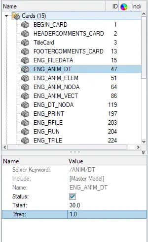
• This will set the number of animation steps during simulation to 30.
• Now we have to set the case for the default and the recommended properties.

• CASE 1 –
• For the first case the properties is to be set for the default values.
• Go to the TAB AREA > PROPERTIES > HAT_SECTION AND CLOSE OUT PANEL, all the element formulation flags are set to the default flag.
• 
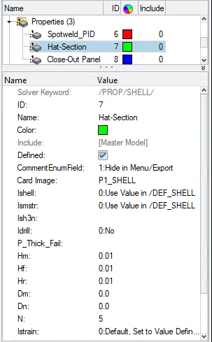
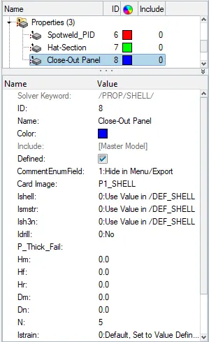
• Now, to run the file go to ANALYSIS > RADIOSS > INPUT FILE > EXPORT OPTIONS = ALL > RUN OPTIONS = ALL > RUN NUMBER = 1 > INCLUDE CONNECTORS > OPTIONS = -NT 4 > RADIOSS.
• 
• This will run the radios file for simulations.
• A window will open and show the status of the run file.
• 
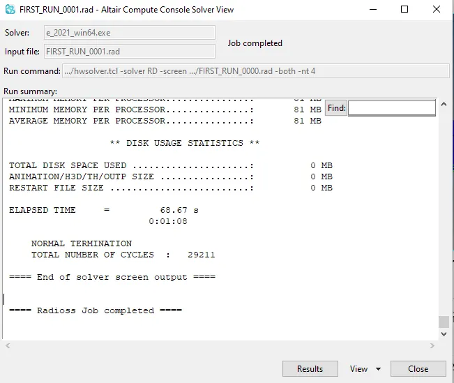
• Once the radioss file is run, open a new window and open Hyperview.
• In Hyperview load the .h3d file and click APPLY.
• Play the simulation to view the deformation or displacement.
• Go to CONTOUR > RESULT TYPE = VOV MISES > AVERAGING METHOD = SIMPLE > APPLY.
• 
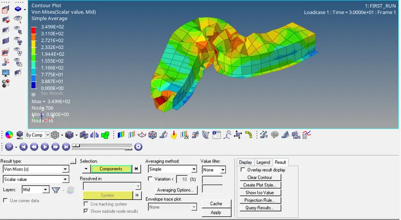
• This will show the vov mises stress on the beam section.
• Now, go to PAGE WINDOW LAYOUT > SIDE BY SIDE.
• This will open other window within the same window.
• Click on the left mouse mutton on the respective window to switch between the windows.
• On the other window open Hypergraph 2D.
• Go to DATA FILE > OPEN > FIRST_RUT01 > OPEN.
• This will open the results file in which the hourglass energy, contact energy, rigid wall forces, etc are saved.
• Go to GLOBAL VARIABLES > INTERNAL ENEGRY > MAG > APPLY. This will plot the internal energy graph.
• 
• Similarly, plot the graphs for Kinetic energy, Contact energy, Hourglass energy, Rigid Wall forces.
• Save the model and the results file.

• CASE 2 –
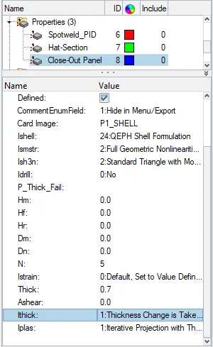
• For the second case the following properties are recommended-
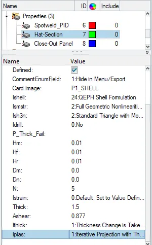
  • Ishell = 24: QEPH 4 nodes shells are best combination of cost and accuracy.
  • Ismstr = 2: Full Geometric nonlinearities with possible small strain formulation.
  • Ish3n = 2: Stranded 3 noded shell (CO) with modification for large rotation.
  • N = 5: Number of integration points set to 5 for accuracy bending.
  • Ithick = 1: Thickness change is taken into account for accuracy.
  • Iplas = 1: Iterative plasticity for good accuracy.
• For this go to TAB AREA > PROPERTIES > HAT_SECTION AND CLOSE_OUT_PANEL and select the above values.
• 
• Now, to run the file go to ANALYSIS > RADIOSS > INPUT FILE > EXPORT OPTIONS = ALL > RUN OPTIONS = ALL > RUN NUMBER = 1 > INCLUDE CONNECTORS > OPTIONS = -NT 4 > RADIOSS.
• 
• This will run the radios file for simulations.
• A window will open and show the status of the run file.
• 
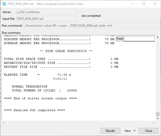
• Once the radioss file is run, open a new window and open Hyperview.
• In Hyperview load the .h3d file and click APPLY.
• Play the simulation to view the deformation or displacement.
• Go to CONTOUR > RESULT TYPE = VOV MISES > AVERAGING METHOD = SIMPLE > APPLY.
• 
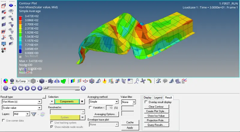
• This will show the vov mises stress on the beam section.
• Now, go to PAGE WINDOW LAYOUT > SIDE BY SIDE.
• This will open other window within the same window.
• Click on the left mouse mutton on the respective window to switch between the windows.
• On the other window open Hypergraph 2D.
• Go to DATA FILE > OPEN > FIRST_RUT01 > OPEN.
• This will open the results file in which the hourglass energy, contact energy, rigid wall forces, etc are saved.
• Go to GLOBAL VARIABLES > INTERNAL ENEGRY > MAG > APPLY. This will plot the internal energy graph.
• 
• Similarly, plot the graphs for Kinetic energy, Contact energy, Hourglass energy, Rigid Wall forces.
• Save the model and the results file.

RESULTS COMPARISION:

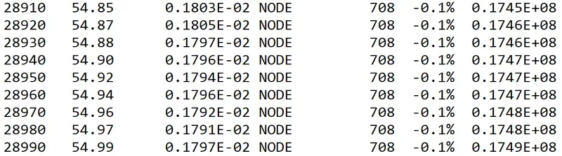
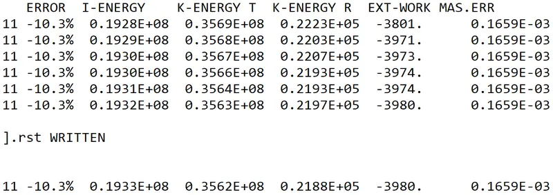
• Energy error –

case 1 - (-10.3%)

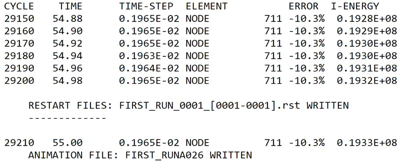
case2- (-0.1%)

• Mass error –

case 1 - (0.1659E-03)

case 2- (0.1659E-03)

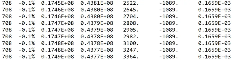
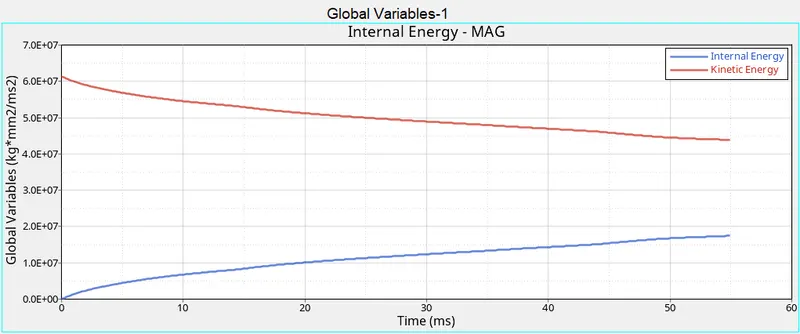
• Internal and Kinetic energy –

case1 - (KE = 3.5E+07; IE = 2.0E+07)

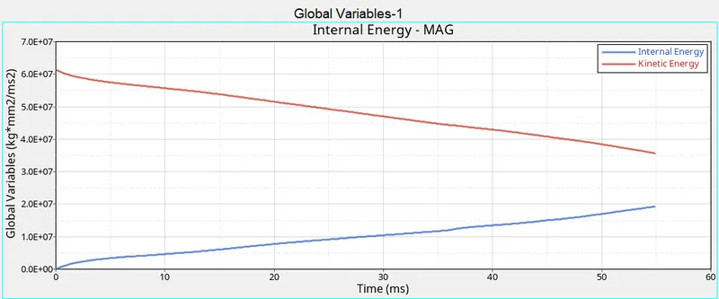
case2 - (KE = 4.4E+07; IE = 1.8E+07)

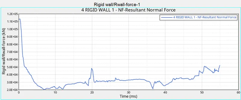
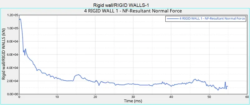
• Normal resultant rigid wall forces –

case1 - (5.3E+04 @55ms)

case 2 - (1.2E+04 @55ms)

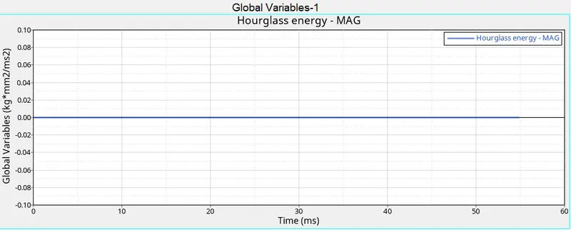
• Hourglass energy -

case 1 - (6.4E+06 @ 55ms)

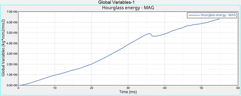
case 2 - (0 @ 55ms)

WHY DID THE RESULTS CHANGE?

Concept of Hourglass:

• The shell elements are solved by using the integration points for each nodal entity.
• The methods include full integration and reduced integration.
• Hourglass is a mode of deformation that occurs in a reduced integration shell elements where no stresses are produced.
• As the stresses are not produced, it reduces the accuracy and true response of the structure.
• This leads to inaccurate strain displacement results within unrealistic deformations.
• In an under-integrated element, displacement and deformation exists for each node of the element.
• If the summation and forces of all these forces and displacements provide zero stress and strain on the integration point, then the element fails to calculate the stiffness for the mode of deformation.
• Thus the element enters into Hourglass.
• To control the Hourglassing we use reduced integration element formulation shell elements.
• Ishell = 1,2,3,4 and Ishell = 24(QEPH) are used.
• Ishell = 24(QEPH) uses 1 no of integration point.
• Ishell = 1,2,3,4 (Q4) employs Perturbation method, whereas Ishell = 24 (QEPH) employs Physical Stabilization for controlling Hourglass.
• Ishell = 24(QEPH), which we used in the second case, shell elements control the Hourglass from the material level.
• Here the Hourglass loading stiffness and Hourglass yield depends on the material properties.
• Being advantage, that it works perfectly well at all kinds of Loading-Unloading cases.
• Ish3n = 2: For tria elements with modification for large rotation, 1 no of integration point on the surface, no Hourglass deformation.
• Ismstr = 2 is a large strain with full geometric non-linearities.
• The phenomena like negative volume generation, large distortion and excessive displacement comes under large deformations.
• Large strain formulation is best suited for non-linear, elastoplastic behavior.
• N = 5: Number of integration points throughout the thickness.
• Ithick =1: the change thickness is not only considered for post-processing, but also used to compute the strain and stresses from true thickness.
• Iplas =1: Iterative projection with three newton interactions (more accurate).
• Hence, due to this we can observe an energy error of only -0.1% in case 2.
• The Hourglass energy in case 2 is observed to be zero.
• Also the Rigid wall forces are much lower in case 2 than in case 1.

LEARNING OUTCOMES:

• Element shell formulation flags.
• Energy error and mass error.
• To run the RADIOSS file.
• To check the Displacement and Stress on the beam in the Hyperview.
• To plot energy and force graphs in HyperGraph 2D.
• To compare the results for different element formulation.
• To read and understand the RADIOSS Run file and Engine file.

CONCLUSION:

• Hence, we conclude that the following Element Formulation Property Flags provide best results than the Default values-

Ishell = 24: QEPH 4 nodes shells are best combination of cost and accuracy.

Ismstr = 2: Full Geometric nonlinearities with possible small strain formulation.

Ish3n = 2: Stranded 3 noded shell (CO) with modification for large rotation.

N = 5: Number of integration points set to 5 for accuracy bending.

Ithick = 1: Thickness change is taken into account for accuracy.

Iplas = 1: Iterative plasticity for good accuracy.